Tree

                                     Tree

Introduction

• Tree is a hierarchical data structure which stores the information naturally in the form of hierarchy style.
• Tree is one of the most powerful and advanced data structures.
• It is a non-linear data structure compared to arrays, linked lists, stack and queue.
• It represents the nodes connected by edges.

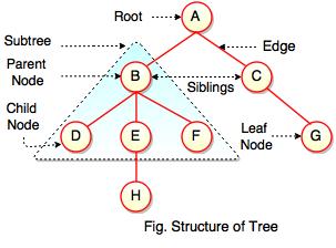
The above figure represents structure of a tree. Tree has 2 subtrees.
A is a parent of B and C.
B is called a child of A and also parent of D, E, F.

Tree is a collection of elements called Nodes, where each node can have arbitrary number of children.

Field	Description
Root	Root is a special node in a tree. The entire tree is referenced through it. It does not have a parent.
Parent Node	Parent node is an immediate predecessor of a node.
Child Node	All immediate successors of a node are its children.
Siblings	Nodes with the same parent are called Siblings.
Path	Path is a number of successive edges from source node to destination node.
Height of Node	Height of a node represents the number of edges on the longest path between that node and a leaf.
Height of Tree	Height of tree represents the height of its root node.
Depth of Node	Depth of a node represents the number of edges from the tree's root node to the node.
Degree of Node	Degree of a node represents a number of children of a node.
Edge	Edge is a connection between one node to another. It is a line between two nodes or a node and a leaf.

In the above figure, D, F, H, G are leaves. B and C are siblings. Each node excluding a root is connected by a direct edge from exactly one other node
parent →  children.

Levels of a node

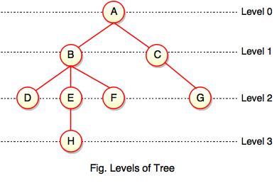
Levels of a node represents the number of connections between the node and the root. It represents generation of a node. If the root node is at level 0, its next node is at level 1, its grand child is at level 2 and so on. Levels of a node can be shown as follows:



Note:

- If node has no children, it is called Leaves or External Nodes.

- Nodes which are not leaves, are called Internal Nodes. Internal nodes have at least one child.

- A tree can be empty with no nodes or a tree consists of one node called the Root.

Height of a Node

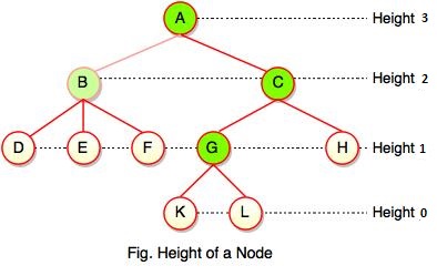
As we studied, height of a node is a number of edges on the longest path between that node and a leaf. Each node has height.

In the above figure, A, B, C, D can have height. Leaf cannot have height as there will be no path starting from a leaf. Node A's height is the number of edges of the path to K not to D. And its height is 3.

Note:

- Height of a node defines the longest path from the node to a leaf.

- Path can only be downward.

Depth of a Node

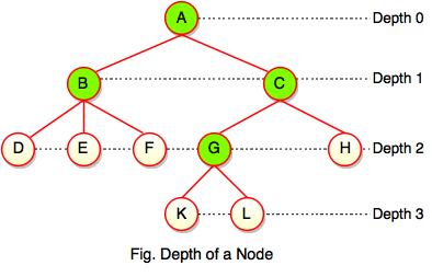
While talking about the height, it locates a node at bottom where for depth, it is located at top which is root level and therefore we call it depth of a node.

In the above figure, Node G's depth is 2. In depth of a node, we just count how many edges between the targeting node & the root and ignoring the directions.

Note: Depth of the root is 0.

Advantages of Tree

• Tree reflects structural relationships in the data.
• It is used to represent hierarchies.
• It provides an efficient insertion and searching operations.
• Trees are flexible. It allows to move subtrees around with minimum effort.

 B-Tree

B-Tree is a self-balancing search tree. In most of the other self-balancing search trees (like AVL and Red-Black Trees), it is assumed that everything is in main memory. To understand the use of B-Trees, we must think of the huge amount of data that cannot fit in main memory. When the number of keys is high, the data is read from disk in the form of blocks. Disk access time is very high compared to main memory access time. The main idea of using B-Trees is to reduce the number of disk accesses. Most of the tree operations (search, insert, delete, max, min, ..etc ) require O(h) disk accesses where h is the height of the tree. B-tree is a fat tree. The height of B-Trees is kept low by putting maximum possible keys in a B-Tree node. Generally, a B-Tree node size is kept equal to the disk block size. Since h is low for B-Tree, total disk accesses for most of the operations are reduced significantly compared to balanced Binary Search Trees like AVL Tree, Red-Black Tree, ..etc.

Properties of B-Tree
1) All leaves are at same level.
2) A B-Tree is defined by the term minimum degree ‘t’. The value of t depends upon disk block size.
3) Every node except root must contain at least t-1 keys. Root may contain minimum 1 key.
4) All nodes (including root) may contain at most 2t – 1 keys.
5) Number of children of a node is equal to the number of keys in it plus 1.
6) All keys of a node are sorted in increasing order. The child between two keys k1 and k2 contains all keys in the range from k1 and k2.
7) B-Tree grows and shrinks from the root which is unlike Binary Search Tree. Binary Search Trees grow downward and also shrink from downward.
8) Like other balanced Binary Search Trees, time complexity to search, insert and delete is O(Logn).

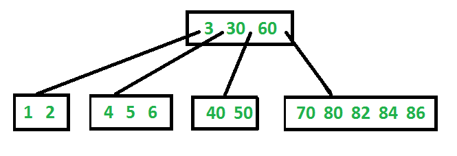
Following is an example B-Tree of minimum degree 3. Note that in practical B-Trees, the value of minimum degree is much more than 3.

Search
Search is similar to the search in Binary Search Tree. Let the key to be searched be k. We start from the root and recursively traverse down. For every visited non-leaf node, if the node has the key, we simply return the node. Otherwise, we recur down to the appropriate child (The child which is just before the first greater key) of the node. If we reach a leaf node and don’t find k in the leaf node, we return NULL.

Traverse
Traversal is also similar to Inorder traversal of Binary Tree. We start from the leftmost child, recursively print the leftmost child, then repeat the same process for remaining children and keys. In the end, recursively print the rightmost child.

Insert Operation in B-Tree

In the previous post, we introduced B-Tree. We also discussed search() and traverse() functions.
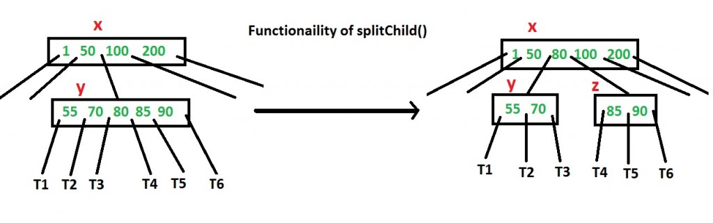
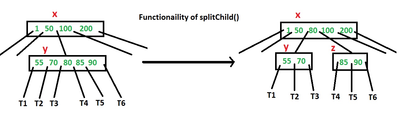
In this post, insert() operation is discussed. A new key is always inserted at the leaf node. Let the key to be inserted be k. Like BST, we start from the root and traverse down till we reach a leaf node. Once we reach a leaf node, we insert the key in that leaf node. Unlike BSTs, we have a predefined range on the number of keys that a node can contain. So before inserting a key to the node, we make sure that the node has extra space.
How to make sure that a node has space available for a key before the key is inserted? We use an operation called splitChild() that is used to split a child of a node. See the following diagram to understand split. In the following diagram, child y of x is being split into two nodes y and z. Note that the splitChild operation moves a key up and this is the reason B-Trees grow up, unlike BSTs which grow down.

As discussed above, to insert a new key, we go down from root to leaf. Before traversing down to a node, we first check if the node is full. If the node is full, we split it to create space. Following is the complete algorithm.

Insertion
1) Initialize x as root.
2) While x is not leaf, do following
..a) Find the child of x that is going to be traversed next. Let the child be y.
..b) If y is not full, change x to point to y.
..c) If y is full, split it and change x to point to one of the two parts of y. If k is smaller than mid key in y, then set x as the first part of y. Else second part of y. When we split y, we move a key from y to its parent x.
3) The loop in step 2 stops when x is leaf. x must have space for 1 extra key as we have been splitting all nodes in advance. So simply insert k to x.

Note that the algorithm follows the Cormen book. It is actually a proactive insertion algorithm where before going down to a node, we split it if it is full. The advantage of splitting before is, we never traverse a node twice. If we don’t split a node before going down to it and split it only if a new key is inserted (reactive), we may end up traversing all nodes again from leaf to root. This happens in cases when all nodes on the path from the root to leaf are full. So when we come to the leaf node, we split it and move a key up. Moving a key up will cause a split in parent node (because the parent was already full). This cascading effect never happens in this proactive insertion algorithm. There is a disadvantage of this proactive insertion though, we may do unnecessary splits.

Let us understand the algorithm with an example tree of minimum degree ‘t’ as 3 and a sequence of integers 10, 20, 30, 40, 50, 60, 70, 80 and 90 in an initially empty B-Tree.

Initially root is NULL. Let us first insert 10.

Let us now insert 20, 30, 40 and 50. They all will be inserted in root because the maximum number of keys a node can accommodate is 2*t – 1 which is 5.

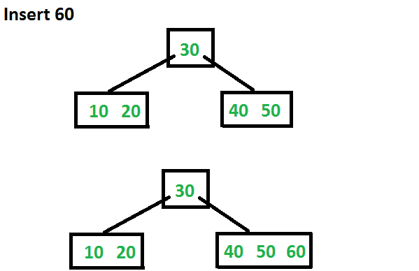
Let us now insert 60. Since root node is full, it will first split into two, then 60 will be inserted into the appropriate child.

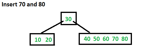
Let us now insert 70 and 80. These new keys will be inserted into the appropriate leaf without any split.

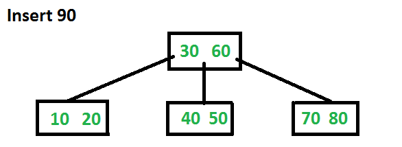
Let us now insert 90. This insertion will cause a split. The middle key will go up to the parent.

Delete Operation in B-Tree

Deletion process:
Deletion from a B-tree is more complicated than insertion, because we can delete a key from any node-not just a leaf—and when we delete a key from an internal node, we will have to rearrange the node’s children.

    As in insertion, we must make sure the deletion doesn’t violate the B-tree properties. Just as we had to ensure that a node didn’t get too big due to insertion, we must ensure that a node doesn’t get too small during deletion (except that the root is allowed to have fewer than the minimum number t-1 of keys). Just as a simple insertion algorithm might have to back up if a node on the path to where the key was to be inserted was full, a simple approach to deletion might have to back up if a node (other than the root) along the path to where the key is to be deleted has the minimum number of keys.

    The deletion procedure deletes the key k from the subtree rooted at x. This procedure guarantees that whenever it calls itself recursively on a node x, the number of keys in x is at least the minimum degree t . Note that this condition requires one more key than the minimum required by the usual B-tree conditions, so that sometimes a key may have to be moved into a child node before recursion descends to that child. This strengthened condition allows us to delete a key from the tree in one downward pass without having to “back up” (with one exception, which we’ll explain). You should interpret the following specification for deletion from a B-tree with the understanding that if the root node x ever becomes an internal node having no keys (this situation can occur in cases 2c and 3b then we delete x, and x’s only child x.c1 becomes the new root of the tree, decreasing the height of the tree by one and preserving the property that the root of the tree contains at least one key (unless the tree is empty).

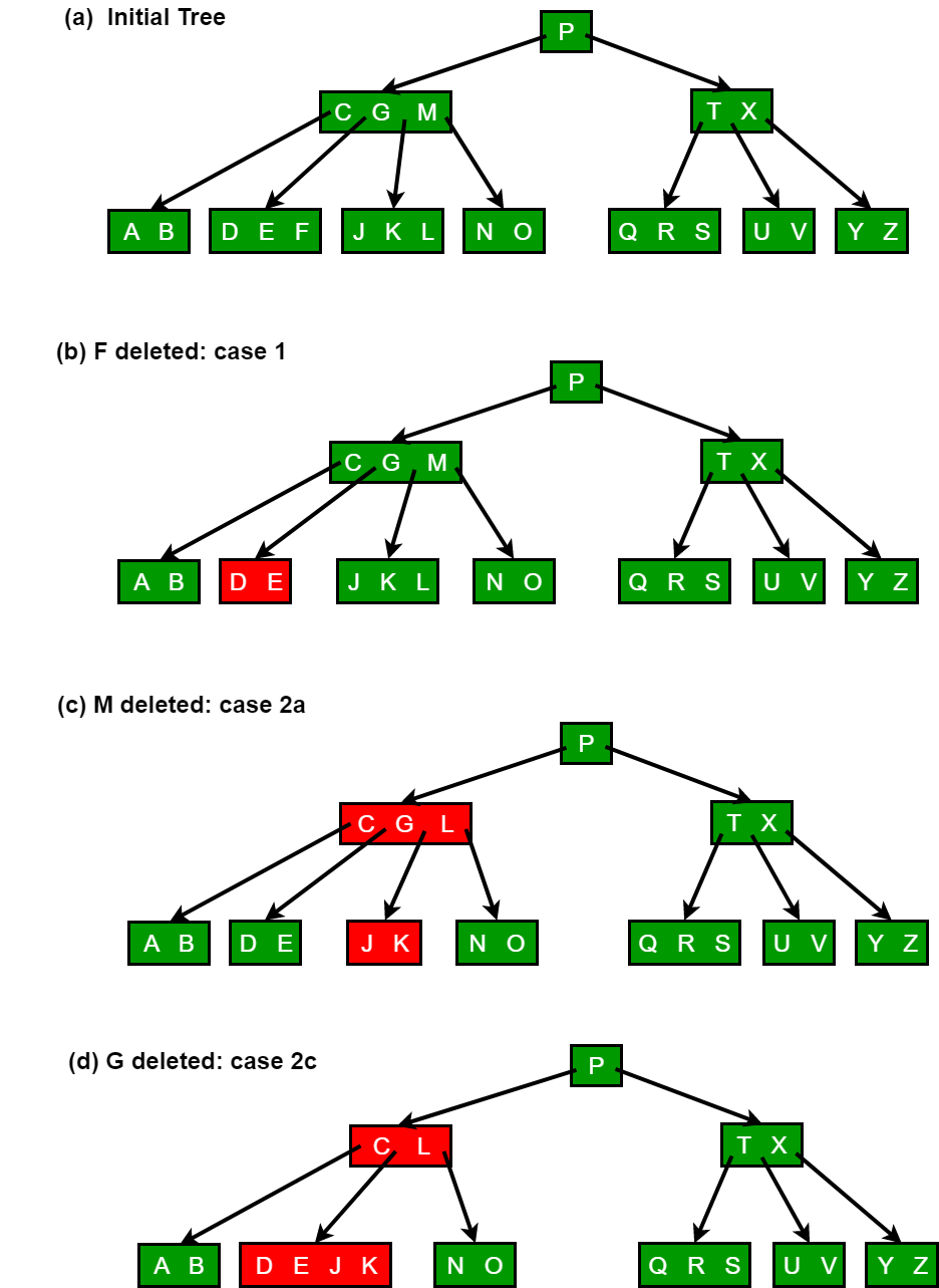
We sketch how deletion works with various cases of deleting keys from a B-tree.

1. If the key k is in node x and x is a leaf, delete the key k from x.

2. If the key k is in node x and x is an internal node, do the following.

    a) If the child y that precedes k in node x has at least t keys, then find the predecessor k0 of k in the sub-tree rooted at y. Recursively delete k0, and replace k by k0 in x. (We can find k0 and delete it in a single downward pass.)

    b) If y has fewer than t keys, then, symmetrically, examine the child z that follows k in node x. If z has at least t keys, then find the successor k0 of k in the subtree rooted at z. Recursively delete k0, and replace k by k0 in x. (We can find k0 and delete it in a single downward pass.)

     c) Otherwise, if both y and z have only t-1 keys, merge k and all of z into y, so that x loses both k and the pointer to z, and y now contains 2t-1 keys. Then free z and recursively delete k from y.

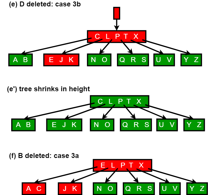
3. If the key k is not present in internal node x, determine the root x.c(i) of the appropriate subtree that must contain k, if k is in the tree at all. If x.c(i) has only t-1 keys, execute step 3a or 3b as necessary to guarantee that we descend to a node containing at least t keys. Then finish by recursing on the appropriate child of x.

    a) If x.c(i) has only t-1 keys but has an immediate sibling with at least t keys, give x.c(i) an extra key by moving a key from x down into x.c(i), moving a key from x.c(i) ’s immediate left or right sibling up into x, and moving the appropriate child pointer from the sibling into x.c(i).

    b) If x.c(i) and both of x.c(i)’s immediate siblings have t-1 keys, merge x.c(i) with one sibling, which involves moving a key from x down into the new merged node to become the median key for that node.

Since most of the keys in a B-tree are in the leaves, deletion operations are most often used to delete keys from leaves. The recursive delete procedure then acts in one downward pass through the tree, without having to back up. When deleting a key in an internal node, however, the procedure makes a downward pass through the tree but may have to return to the node from which the key was deleted to replace the key with its predecessor or successor (cases 2a and 2b).

The following figures explain the deletion process.

Red Black Tree

A Red Black Tree is a category of the self-balancing binary search tree. It was created in 1972 by Rudolf Bayer who termed them "symmetric binary B-trees."

A red-black tree is a Binary tree where a particular node has color as an extra attribute, either red or black. By check the node colors on any simple path from the root to a leaf, red-black trees secure that no such path is higher than twice as long as any other so that the tree is generally balanced.

Properties of Red-Black Trees

A red-black tree must satisfy these properties:

1. The root is always black.
2. A nil is recognized to be black. This factor that every non-NIL node has two children.
3. Black Children Rule: The children of any red node are black.
4. Black Height Rule: For particular node v, there exists an integer bh (v) such that specific downward path from v to a nil has correctly bh (v) black real (i.e. non-nil) nodes. Call this portion the black height of v. We determine the black height of an RB tree to be the black height of its root.

A tree T is an almost red-black tree (ARB tree) if the root is red, but other conditions above hold.

Operations on RB Trees:

The search-tree operations TREE-INSERT and TREE-DELETE, when runs on a red-black tree with n keys, take O (log n) time. Because they customize the tree, the conclusion may violate the red-black properties. To restore these properties, we must change the color of some of the nodes in the tree and also change the pointer structure.

1. Rotation:

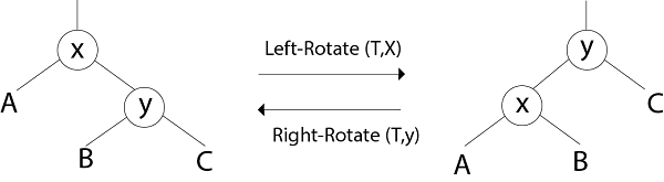
Restructuring operations on red-black trees can generally be expressed more clearly in details of the rotation operation.

Clearly, the order (Ax By C) is preserved by the rotation operation. Therefore, if we start with a BST and only restructure using rotation, then we will still have a BST i.e. rotation do not break the BST-Property.

LEFT ROTATE (T, x)
 1. y ← right [x]
 1. y ← right [x]
 2. right [x] ← left [y]
 3. p [left[y]] ← x
 4. p[y] ← p[x]
 5. If p[x] = nil [T]
   then root [T] ← y
    else if x = left [p[x]]          
      then left [p[x]] ← y
    else right [p[x]] ← y
 6. left [y] ← x.
 7. p [x] ← y. 

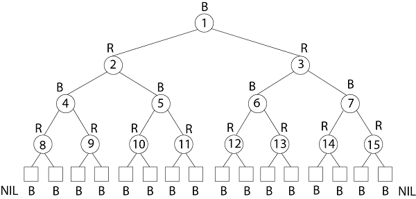
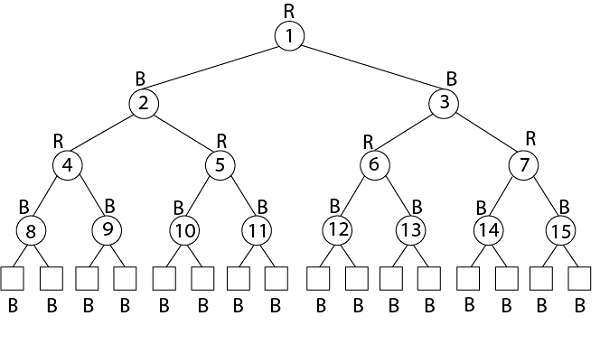
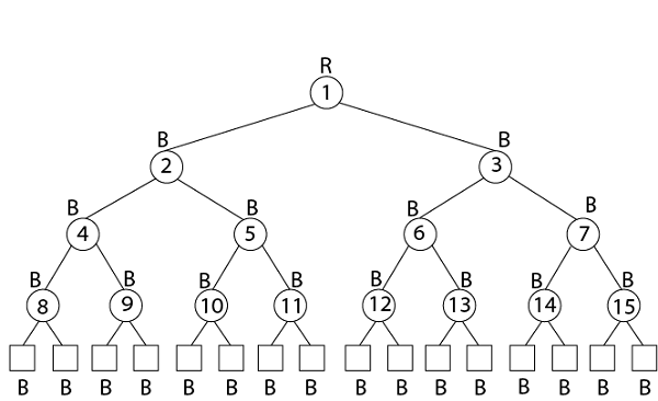
Example: Draw the complete binary tree of height 3 on the keys {1, 2, 3... 15}. Add the NIL leaves and color the nodes in three different ways such that the black heights of the resulting trees are: 2, 3 and 4.

Solution:

Tree with black-height-2

Tree with black-height-3

Tree with black-height-4

---

2. Insertion:

• Insert the new node the way it is done in Binary Search Trees.
• Color the node red
• If an inconsistency arises for the red-black tree, fix the tree according to the type of discrepancy.

A discrepancy can decision from a parent and a child both having a red color. This type of discrepancy is determined by the location of the node concerning grandparent, and the color of the sibling of the parent.

RB-INSERT (T, z)
 1. y ← nil [T]
 2. x ← root [T]
 3. while x ≠ NIL [T]
 4. do y ← x
 5. if key [z] < key [x]
 6. then x  ← left [x]
 7. else x ←  right [x]
 8. p [z] ← y
 9. if y = nil [T]
 10. then root [T] ← z
 11. else if key [z] < key [y]
 12. then left [y] ← z
 13. else right [y] ← z
 14. left [z] ← nil [T]
 15. right [z] ← nil [T]
 16. color [z] ← RED
 17. RB-INSERT-FIXUP (T, z)

After the insert new node, Coloring this new node into black may violate the black-height conditions and coloring this new node into red may violate coloring conditions i.e. root is black and red node has no red children. We know the black-height violations are hard. So we color the node red. After this, if there is any color violation, then we have to correct them by an RB-INSERT-FIXUP procedure.

RB-INSERT-FIXUP (T, z)
 1. while color [p[z]] = RED
 2. do if p [z] = left [p[p[z]]]
 3. then y ← right [p[p[z]]]
 4. If color [y] = RED
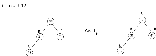
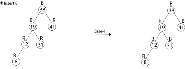
 5. then color [p[z]] ← BLACK    //Case 1
 6. color [y] ← BLACK            //Case 1
 7. color [p[z]] ← RED           //Case 1
 8. z  ← p[p[z]]                 //Case 1
 9. else if z= right [p[z]]
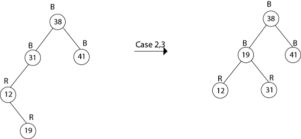
 10. then z ← p [z]              //Case 2
 11. LEFT-ROTATE (T, z)          //Case 2
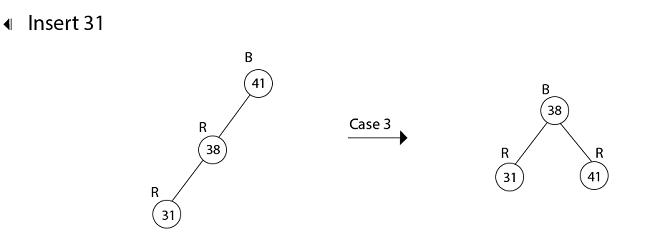
 12. color [p[z]] ← BLACK        //Case 3
 13. color [p [p[z]]] ← RED      //Case 3
 14. RIGHT-ROTATE  (T,p [p[z]])  //Case 3
 15. else (same as then clause)
      With "right" and "left" exchanged
 16. color [root[T]] ← BLACK

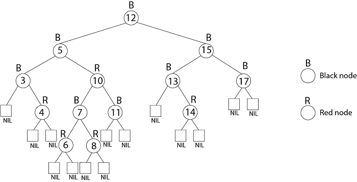
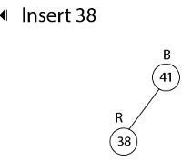
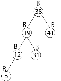
Example: Show the red-black trees that result after successively inserting the keys 41,38,31,12,19,8 into an initially empty red-black tree.

Solution:

Insert 41

Insert 19

Thus the final tree is

---

3. Deletion:

First, search for an element to be deleted

• If the element to be deleted is in a node with only left child, swap this node with one containing the largest element in the left subtree. (This node has no right child).
• If the element to be deleted is in a node with only right child, swap this node with the one containing the smallest element in the right subtree (This node has no left child).
• If the element to be deleted is in a node with both a left child and a right child, then swap in any of the above two ways. While swapping, swap only the keys but not the colors.
• The item to be deleted is now having only a left child or only a right child. Replace this node with its sole child. This may violate red constraints or black constraint. Violation of red constraints can be easily fixed.
• If the deleted node is black, the black constraint is violated. The elimination of a black node y causes any path that contained y to have one fewer black node.
• Two cases arise:
  • The replacing node is red, in which case we merely color it black to make up for the loss of one black node.
  • The replacing node is black.

The strategy RB-DELETE is a minor change of the TREE-DELETE procedure. After splicing out a node, it calls an auxiliary procedure RB-DELETE-FIXUP that changes colors and performs rotation to restore the red-black properties.

RB-DELETE (T, z)
 1. if left [z] = nil [T] or right [z] = nil [T]
 2. then y ← z
 3. else y ← TREE-SUCCESSOR (z)
 4. if left [y] ≠ nil [T]
 5. then x ← left [y]
 6. else x ← right [y]
 7. p [x] ←  p [y]
 8. if p[y] = nil [T]
 9. then root [T]  ← x
 10. else if y = left [p[y]]
 11. then left [p[y]] ← x
 12. else right [p[y]] ← x
 13. if y≠ z
 14. then key [z] ← key [y]
 15. copy y's satellite data into z
 16. if color [y] = BLACK
 17. then RB-delete-FIXUP (T, x)
 18. return y

RB-DELETE-FIXUP (T, x)
 1. while x ≠ root [T] and color [x] = BLACK
 2. do if x = left [p[x]]
 3. then w ← right [p[x]]
 4. if color [w] = RED
 5. then color [w] ← BLACK        //Case 1
 6. color [p[x]] ← RED            //Case 1
 7. LEFT-ROTATE (T, p [x])        //Case 1
 8. w ← right [p[x]]              //Case 1
 9. If color [left [w]] = BLACK and color [right[w]] = BLACK
 10. then color [w] ← RED         //Case 2
 11. x ← p[x]                     //Case 2
 12. else if color [right [w]] = BLACK
 13. then color [left[w]] ← BLACK //Case 3
 14. color [w] ← RED              //Case 3
 15. RIGHT-ROTATE (T, w)          //Case 3
 16. w ← right [p[x]]             //Case 3
 17. color [w] ← color [p[x]]     //Case 4
 18. color p[x] ← BLACK           //Case 4
 19. color [right [w]] ← BLACK    //Case 4
 20. LEFT-ROTATE (T, p [x])       //Case 4
 21. x ← root [T]                 //Case 4
 22. else (same as then clause with "right" and "left" exchanged)
 23. color [x] ← BLACK

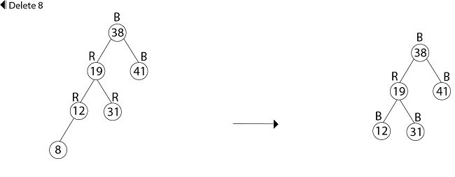
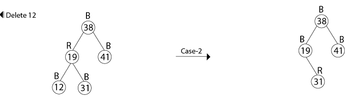
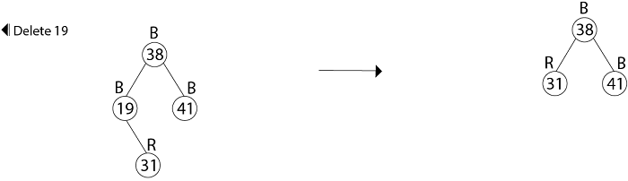
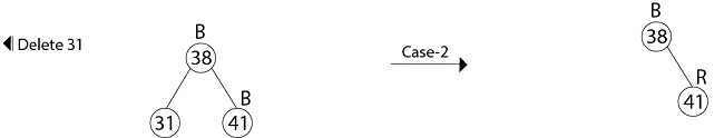
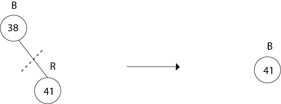
Example: In a previous example, we found that the red-black tree that results from successively inserting the keys 41,38,31,12,19,8 into an initially empty tree. Now show the red-black trees that result from the successful deletion of the keys in the order 8, 12, 19,31,38,41.

Solution:

Delete 38

Delete 41

No Tree

Thank you,

by Er.Shejwal Shrikant.

30-12-2019 Monday.