Branch and Bound
Branch and Bound
Introduction
Introduction
Let us explore all approaches for this problem.
- A Greedy approach is to pick the items in decreasing order of value per unit weight. The Greedy approach works only for fractional knapsack problem and may not produce correct result for 0/1 knapsack.
- We can use Dynamic Programming (DP) for 0/1 Knapsack problem. In DP, we use a 2D table of size n x W. The DP Solution doesn’t work if item weights are not integers.
- Since DP solution doesn’t alway work, a solution is to use Brute Force. With n items, there are 2n solutions to be generated, check each to see if they satisfy the constraint, save maximum solution that satisfies constraint. This solution can be expressed as tree.

- We can use Backtracking to optimize the Brute Force solution. In the tree representation, we can do DFS of tree. If we reach a point where a solution no longer is feasible, there is no need to continue exploring. In the given example, backtracking would be much more effective if we had even more items or a smaller knapsack capacity.

Branch and Bound
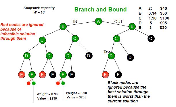
The backtracking based solution works better than brute force by ignoring infeasible solutions. We can do better (than backtracking) if we know a bound on best possible solution subtree rooted with every node. If the best in subtree is worse than current best, we can simply ignore this node and its subtrees. So we compute bound (best solution) for every node and compare the bound with current best solution before exploring the node.
Example bounds used in below diagram are, A down can give $315, B down can $275, C down can $225, D down can $125 and E down can $30. In the next article, we have discussed the process to get these bounds.
 Branch and bound is very useful technique for searching a solution but in worst case, we need to fully calculate the entire tree. At best, we only need to fully calculate one path through the tree and prune the rest of it.
Branch and bound is an algorithm design paradigm which is generally used for solving combinatorial optimization problems. These problems typically exponential in terms of time complexity and may require exploring all possible permutations in worst case. Branch and Bound solve these problems relatively quickly.
Let us consider below 0/1 Knapsack problem to understand Branch and Bound.
Given two integer arrays val[0..n-1] and wt[0..n-1] that represent values and weights associated with n items respectively. Find out the maximum value subset of val[] such that sum of the weights of this subset is smaller than or equal to Knapsack capacity W.
Let us explore all approaches for this problem.
- A Greedy approach is to pick the items in decreasing order of value per unit weight. The Greedy approach works only for fractional knapsack problem and may not produce correct result for 0/1 knapsack.
- We can use Dynamic Programming (DP) for 0/1 Knapsack problem. In DP, we use a 2D table of size n x W. The DP Solution doesn’t work if item weights are not integers.
- Since DP solution doesn’t alway work, a solution is to use Brute Force. With n items, there are 2n solutions to be generated, check each to see if they satisfy the constraint, save maximum solution that satisfies constraint. This solution can be expressed as tree.
- We can use Backtracking to optimize the Brute Force solution. In the tree representation, we can do DFS of tree. If we reach a point where a solution no longer is feasible, there is no need to continue exploring. In the given example, backtracking would be much more effective if we had even more items or a smaller knapsack capacity.
The backtracking based solution works better than brute force by ignoring infeasible solutions. We can do better (than backtracking) if we know a bound on best possible solution subtree rooted with every node. If the best in subtree is worse than current best, we can simply ignore this node and its subtrees. So we compute bound (best solution) for every node and compare the bound with current best solution before exploring the node.
Example bounds used in below diagram are, A down can give $315, B down can $275, C down can $225, D down can $125 and E down can $30. In the next article, we have discussed the process to get these bounds.
Branch and bound is very useful technique for searching a solution but in worst case, we need to fully calculate the entire tree. At best, we only need to fully calculate one path through the tree and prune the rest of it.
Traveling Salesman Problem using Branch And Bound
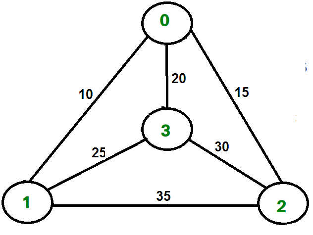
Given a set of cities and distance between every pair of cities, the problem is to find the shortest possible tour that visits every city exactly once and returns to the starting point.
For example, consider the graph shown in figure on right side. A TSP tour in the graph is 0-1-3-2-0. The cost of the tour is 10+25+30+15 which is 80.
Branch and Bound Solution
As seen in the previous articles, in Branch and Bound method, for current node in tree, we compute a bound on best possible solution that we can get if we down this node. If the bound on best possible solution itself is worse than current best (best computed so far), then we ignore the subtree rooted with the node.
As seen in the previous articles, in Branch and Bound method, for current node in tree, we compute a bound on best possible solution that we can get if we down this node. If the bound on best possible solution itself is worse than current best (best computed so far), then we ignore the subtree rooted with the node.
Note that the cost through a node includes two costs.
1) Cost of reaching the node from the root (When we reach a node, we have this cost computed)
2) Cost of reaching an answer from current node to a leaf (We compute a bound on this cost to decide whether to ignore subtree with this node or not).
1) Cost of reaching the node from the root (When we reach a node, we have this cost computed)
2) Cost of reaching an answer from current node to a leaf (We compute a bound on this cost to decide whether to ignore subtree with this node or not).
- In cases of a maximization problem, an upper bound tells us the maximum possible solution if we follow the given node. For example in 0/1 knapsack we used Greedy approach to find an upper bound.
- In cases of a minimization problem, a lower bound tells us the minimum possible solution if we follow the given node. For example, in Job Assignment Problem, we get a lower bound by assigning least cost job to a worker.
In branch and bound, the challenging part is figuring out a way to compute a bound on best possible solution. Below is an idea used to compute bounds for Traveling salesman problem.
Cost of any tour can be written as below.
Cost of a tour T = (1/2) * ∑ (Sum of cost of two edges
                              adjacent to u and in the
                              tour T)
                   where u ∈ V
For every vertex u, if we consider two edges through it in T,
and sum their costs.  The overall sum for all vertices would
be twice of cost of tour T (We have considered every edge
twice.)

(Sum of two tour edges adjacent to u) >= (sum of minimum weight
                                          two edges adjacent to
                                          u)

Cost of any tour >=  1/2) * ∑ (Sum of cost of two minimum
                              weight edges adjacent to u)
                   where u ∈ V
For example, consider the above shown graph. Below are minimum cost two edges adjacent to every node.
Node     Least cost edges   Total cost
0     (0, 1), (0, 2)            25
1     (0, 1), (1, 3)         35
2    (0, 2), (2, 3)            45
3     (0, 3), (1, 3)            45

Thus a lower bound on the cost of any tour =
         1/2(25 + 35 + 45 + 45)
       = 75
Refer this for one more example.
Now we have an idea about computation of lower bound. Let us see how to how to apply it state space search tree. We start enumerating all possible nodes (preferably in lexicographical order)
1. The Root Node: Without loss of generality, we assume we start at vertex “0” for which the lower bound has been calculated above.
Dealing with Level 2: The next level enumerates all possible vertices we can go to (keeping in mind that in any path a vertex has to occur only once) which are, 1, 2, 3… n (Note that the graph is complete). Consider we are calculating for vertex 1, Since we moved from 0 to 1, our tour has now included the edge 0-1. This allows us to make necessary changes in the lower bound of the root.
Lower Bound for vertex 1 =
   Old lower bound - ((minimum edge cost of 0 +
                    minimum edge cost of 1) / 2)
                  + (edge cost 0-1)
How does it work? To include edge 0-1, we add the edge cost of 0-1, and subtract an edge weight such that the lower bound remains as tight as possible which would be the sum of the minimum edges of 0 and 1 divided by 2. Clearly, the edge subtracted can’t be smaller than this.
Dealing with other levels: As we move on to the next level, we again enumerate all possible vertices. For the above case going further after 1, we check out for 2, 3, 4, …n.
Consider lower bound for 2 as we moved from 1 to 1, we include the edge 1-2 to the tour and alter the new lower bound for this node.
Consider lower bound for 2 as we moved from 1 to 1, we include the edge 1-2 to the tour and alter the new lower bound for this node.
Lower bound(2) =
     Old lower bound - ((second minimum edge cost of 1 +
                         minimum edge cost of 2)/2)
                     + edge cost 1-2)
Note: The only change in the formula is that this time we have included second minimum edge cost for 1, because the minimum edge cost has already been subtracted in previous level.
Thank you,
Er. Shejwal Shrikant.
30-12-2019 Monday
Difference between backtracking & Branch and Bound
Backtracking:
* It is used to find all posible solution available to the problem
*It traverse tree by DFS(Depth first Search)
*It realizes that it has made a bad choice & ubndoes the last choice by tracking up.
*It search the state space tree until it found a solution
*It involves feasibility function
Branch-and-Bound(BB):
*It is used to solve optimization problem
*It may traverse the tree in any manner, DFS or BFS
*It realizes that is already has a better optional solution that the pre-solution leads to so it abandons that pre-solution.
*It completely search the state space tree to get optional solution.
*It involves bounding function.
Thank you,
Er. Shejwal Shrikant.
30-12-2019 Monday

Comments
Post a Comment