Processes and CPU Scheduling

               Processes and CPU Scheduling

Process concept

A process is basically a program in execution. The execution of a process must progress in a sequential fashion.

A process is defined as an entity which represents the basic unit of work to be implemented in the system.

To put it in simple terms, we write our computer programs in a text file and when we execute this program, it becomes a process which performs all the tasks mentioned in the program.

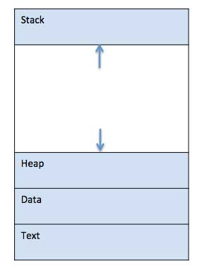
When a program is loaded into the memory and it becomes a process, it can be divided into four sections ─ stack, heap, text and data. The following image shows a simplified layout of a process inside main memory −

S.N.	Component & Description
1	Stack The process Stack contains the temporary data such as method/function parameters, return address and local variables.
2	Heap This is dynamically allocated memory to a process during its run time.
3	Text This includes the current activity represented by the value of Program Counter and the contents of the processor's registers.
4	Data This section contains the global and static variables.

Program

A program is a piece of code which may be a single line or millions of lines. A computer program is usually written by a computer programmer in a programming language. For example, here is a simple program written in C programming language −

#include <stdio.h>

int main() {
   printf("Hello, World! \n");
   return 0;
}

A computer program is a collection of instructions that performs a specific task when executed by a computer. When we compare a program with a process, we can conclude that a process is a dynamic instance of a computer program.

A part of a computer program that performs a well-defined task is known as an algorithm. A collection of computer programs, libraries and related data are referred to as a software.

Process Life Cycle

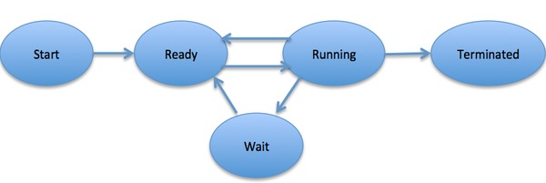
When a process executes, it passes through different states. These stages may differ in different operating systems, and the names of these states are also not standardized.

In general, a process can have one of the following five states at a time.

S.N.	State & Description
1	Start This is the initial state when a process is first started/created.
2	Ready The process is waiting to be assigned to a processor. Ready processes are waiting to have the processor allocated to them by the operating system so that they can run. Process may come into this state after Start state or while running it by but interrupted by the scheduler to assign CPU to some other process.
3	Running Once the process has been assigned to a processor by the OS scheduler, the process state is set to running and the processor executes its instructions.
4	Waiting Process moves into the waiting state if it needs to wait for a resource, such as waiting for user input, or waiting for a file to become available.
5	Terminated or Exit Once the process finishes its execution, or it is terminated by the operating system, it is moved to the terminated state where it waits to be removed from main memory.

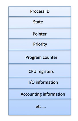
Process Control Block (PCB)

A Process Control Block is a data structure maintained by the Operating System for every process. The PCB is identified by an integer process ID (PID). A PCB keeps all the information needed to keep track of a process as listed below in the table −

S.N.	Information & Description
1	Process State The current state of the process i.e., whether it is ready, running, waiting, or whatever.
2	Process privileges This is required to allow/disallow access to system resources.
3	Process ID Unique identification for each of the process in the operating system.
4	Pointer A pointer to parent process.
5	Program Counter Program Counter is a pointer to the address of the next instruction to be executed for this process.
6	CPU registers Various CPU registers where process need to be stored for execution for running state.
7	CPU Scheduling Information Process priority and other scheduling information which is required to schedule the process.
8	Memory management information This includes the information of page table, memory limits, Segment table depending on memory used by the operating system.
9	Accounting information This includes the amount of CPU used for process execution, time limits, execution ID etc.
10	IO status information This includes a list of I/O devices allocated to the process.

The architecture of a PCB is completely dependent on Operating System and may contain different information in different operating systems. Here is a simplified diagram of a PCB −

The PCB is maintained for a process throughout its lifetime, and is deleted once the process terminates.

Process Scheduling

Definition

The process scheduling is the activity of the process manager that handles the removal of the running process from the CPU and the selection of another process on the basis of a particular strategy.

Process scheduling is an essential part of a Multiprogramming operating systems. Such operating systems allow more than one process to be loaded into the executable memory at a time and the loaded process shares the CPU using time multiplexing.

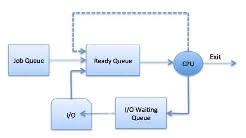
Process Scheduling Queues

The OS maintains all PCBs in Process Scheduling Queues. The OS maintains a separate queue for each of the process states and PCBs of all processes in the same execution state are placed in the same queue. When the state of a process is changed, its PCB is unlinked from its current queue and moved to its new state queue.

The Operating System maintains the following important process scheduling queues −

• Job queue − This queue keeps all the processes in the system.
• Ready queue − This queue keeps a set of all processes residing in main memory, ready and waiting to execute. A new process is always put in this queue.
• Device queues − The processes which are blocked due to unavailability of an I/O device constitute this queue.

The OS can use different policies to manage each queue (FIFO, Round Robin, Priority, etc.). The OS scheduler determines how to move processes between the ready and run queues which can only have one entry per processor core on the system; in the above diagram, it has been merged with the CPU.

Two-State Process Model

Two-state process model refers to running and non-running states which are described below −

S.N.	State & Description
1	Running When a new process is created, it enters into the system as in the running state.
2	Not Running Processes that are not running are kept in queue, waiting for their turn to execute. Each entry in the queue is a pointer to a particular process. Queue is implemented by using linked list. Use of dispatcher is as follows. When a process is interrupted, that process is transferred in the waiting queue. If the process has completed or aborted, the process is discarded. In either case, the dispatcher then selects a process from the queue to execute.

Schedulers

Schedulers are special system software which handle process scheduling in various ways. Their main task is to select the jobs to be submitted into the system and to decide which process to run. Schedulers are of three types −

• Long-Term Scheduler
• Short-Term Scheduler
• Medium-Term Scheduler

Long Term Scheduler

It is also called a job scheduler. A long-term scheduler determines which programs are admitted to the system for processing. It selects processes from the queue and loads them into memory for execution. Process loads into the memory for CPU scheduling.

The primary objective of the job scheduler is to provide a balanced mix of jobs, such as I/O bound and processor bound. It also controls the degree of multiprogramming. If the degree of multiprogramming is stable, then the average rate of process creation must be equal to the average departure rate of processes leaving the system.

On some systems, the long-term scheduler may not be available or minimal. Time-sharing operating systems have no long term scheduler. When a process changes the state from new to ready, then there is use of long-term scheduler.

Short Term Scheduler

It is also called as CPU scheduler. Its main objective is to increase system performance in accordance with the chosen set of criteria. It is the change of ready state to running state of the process. CPU scheduler selects a process among the processes that are ready to execute and allocates CPU to one of them.

Short-term schedulers, also known as dispatchers, make the decision of which process to execute next. Short-term schedulers are faster than long-term schedulers.

Medium Term Scheduler

Medium-term scheduling is a part of swapping. It removes the processes from the memory. It reduces the degree of multiprogramming. The medium-term scheduler is in-charge of handling the swapped out-processes.

A running process may become suspended if it makes an I/O request. A suspended processes cannot make any progress towards completion. In this condition, to remove the process from memory and make space for other processes, the suspended process is moved to the secondary storage. This process is called swapping, and the process is said to be swapped out or rolled out. Swapping may be necessary to improve the process mix.

Comparison among Scheduler

S.N.	Long-Term Scheduler	Short-Term Scheduler	Medium-Term Scheduler
1	It is a job scheduler	It is a CPU scheduler	It is a process swapping scheduler.
2	Speed is lesser than short term scheduler	Speed is fastest among other two	Speed is in between both short and long term scheduler.
3	It controls the degree of multiprogramming	It provides lesser control over degree of multiprogramming	It reduces the degree of multiprogramming.
4	It is almost absent or minimal in time sharing system	It is also minimal in time sharing system	It is a part of Time sharing systems.
5	It selects processes from pool and loads them into memory for execution	It selects those processes which are ready to execute	It can re-introduce the process into memory and execution can be continued.

Context Switch

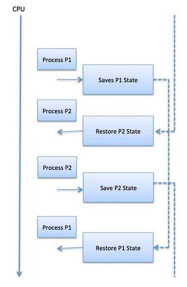
A context switch is the mechanism to store and restore the state or context of a CPU in Process Control block so that a process execution can be resumed from the same point at a later time. Using this technique, a context switcher enables multiple processes to share a single CPU. Context switching is an essential part of a multitasking operating system features.

When the scheduler switches the CPU from executing one process to execute another, the state from the current running process is stored into the process control block. After this, the state for the process to run next is loaded from its own PCB and used to set the PC, registers, etc. At that point, the second process can start executing.

Context switches are computationally intensive since register and memory state must be saved and restored. To avoid the amount of context switching time, some hardware systems employ two or more sets of processor registers. When the process is switched, the following information is stored for later use.

• Program Counter
• Scheduling information
• Base and limit register value
• Currently used register
• Changed State
• I/O State information
• Accounting information

Operation on process

There are many operations that can be performed on processes. Some of these are process creation, process preemption, process blocking, and process termination. These are given in detail as follows:

1. Process Creation

Processes need to be created in the system for different operations. This can be done by the following events:

• User request for process creation
• System initialization
• Execution of a process creation system call by a running process
• Batch job initialization

A process may be created by another process using fork(). The creating process is called the parent process and the created process is the child process. A child process can have only one parent but a parent process may have many children. Both the parent and child processes have the same memory image, open files, and environment strings. However, they have distinct address spaces.

A diagram that demonstrates process creation using fork() is as follows:

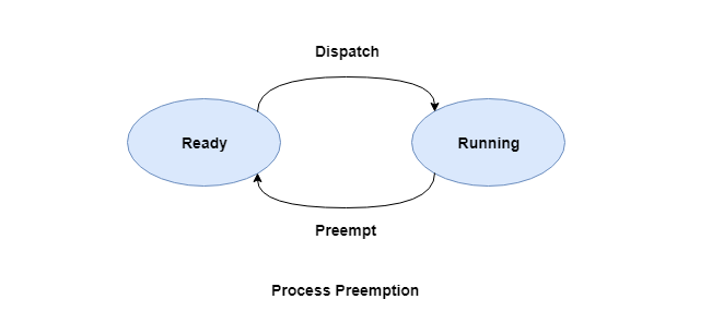
2. Process Preemption

An interrupt mechanism is used in preemption that suspends the process executing currently and the next process to execute is determined by the short-term scheduler. Preemption makes sure that all processes get some CPU time for execution.

A diagram that demonstrates process preemption is as follows:

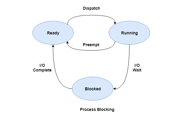
3. Process Blocking

The process is blocked if it is waiting for some event to occur. This event may be I/O as the I/O events are executed in the main memory and don't require the processor. After the event is complete, the process again goes to the ready state.

A diagram that demonstrates process blocking is as follows:

4. Process Termination

After the process has completed the execution of its last instruction, it is terminated. The resources held by a process are released after it is terminated.

A child process can be terminated by its parent process if its task is no longer relevant. The child process sends its status information to the parent process before it terminates. Also, when a parent process is terminated, its child processes are terminated as well as the child processes cannot run if the parent processes are terminated.

Cooperating processes are those that can affect or are affected by other processes running on the system. Cooperating processes may share data with each other.

Reasons for needing cooperating processes

There may be many reasons for the requirement of cooperating processes. Some of these are given as follows:

1. Modularity
Modularity involves dividing complicated tasks into smaller subtasks. These subtasks can completed by different cooperating processes. This leads to faster and more efficient completion of the required tasks.
2. Information Sharing
Sharing of information between multiple processes can be accomplished using cooperating processes. This may include access to the same files. A mechanism is required so that the processes can access the files in parallel to each other.
3. Convenience
There are many tasks that a user needs to do such as compiling, printing, editing etc. It is convenient if these tasks can be managed by cooperating processes.
4. Computation Speedup
Subtasks of a single task can be performed parallely using cooperating processes. This increases the computation speedup as the task can be executed faster. However, this is only possible if the system has multiple processing elements.

 Cooperation processes

Cooperating processes can coordinate with each other using shared data or messages. Details about these are given as follows:

1. Cooperation by Sharing
The cooperating processes can cooperate with each other using shared data such as memory, variables, files, databases etc. Critical section is used to provide data integrity and writing is mutually exclusive to prevent inconsistent data.
A diagram that demonstrates cooperation by sharing is given as follows:

In the above diagram, Process P1 and P2 can cooperate with each other using shared data such as memory, variables, files, databases etc.
2. Cooperation by Communication
The cooperating processes can cooperate with each other using messages. This may lead to deadlock if each process is waiting for a message from the other to perform a operation. Starvation is also possible if a process never receives a message.
A diagram that demonstrates cooperation by communication is given as follows:

In the above diagram, Process P1 and P2 can cooperate with each other using messages to communicate.

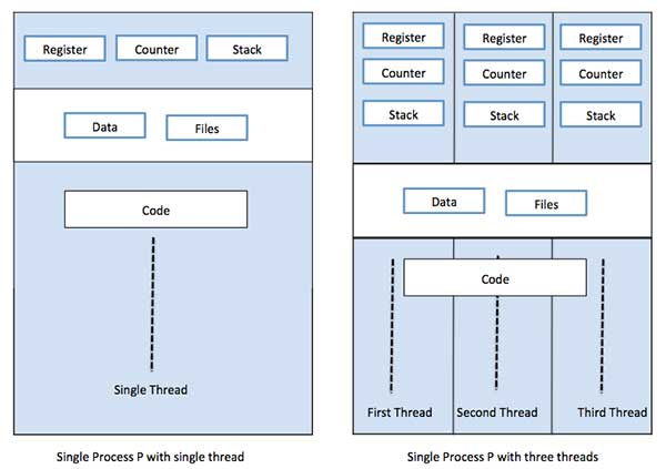
Thread

A thread is a flow of execution through the process code, with its own program counter that keeps track of which instruction to execute next, system registers which hold its current working variables, and a stack which contains the execution history.

A thread shares with its peer threads few information like code segment, data segment and open files. When one thread alters a code segment memory item, all other threads see that.

A thread is also called a lightweight process. Threads provide a way to improve application performance through parallelism. Threads represent a software approach to improving performance of operating system by reducing the overhead thread is equivalent to a classical process.

Each thread belongs to exactly one process and no thread can exist outside a process. Each thread represents a separate flow of control. Threads have been successfully used in implementing network servers and web server. They also provide a suitable foundation for parallel execution of applications on shared memory multiprocessors. The following figure shows the working of a single-threaded and a multithreaded process.

Difference between Process and Thread

S.N.	Process	Thread
1	Process is heavy weight or resource intensive.	Thread is light weight, taking lesser resources than a process.
2	Process switching needs interaction with operating system.	Thread switching does not need to interact with operating system.
3	In multiple processing environments, each process executes the same code but has its own memory and file resources.	All threads can share same set of open files, child processes.
4	If one process is blocked, then no other process can execute until the first process is unblocked.	While one thread is blocked and waiting, a second thread in the same task can run.
5	Multiple processes without using threads use more resources.	Multiple threaded processes use fewer resources.
6	In multiple processes each process operates independently of the others.	One thread can read, write or change another thread's data.

Advantages of Thread

• Threads minimize the context switching time.
• Use of threads provides concurrency within a process.
• Efficient communication.
• It is more economical to create and context switch threads.
• Threads allow utilization of multiprocessor architectures to a greater scale and efficiency.

Types of Thread

Threads are implemented in following two ways −

• User Level Threads − User managed threads.
• Kernel Level Threads − Operating System managed threads acting on kernel, an operating system core.

User Level Threads

In this case, the thread management kernel is not aware of the existence of threads. The thread library contains code for creating and destroying threads, for passing message and data between threads, for scheduling thread execution and for saving and restoring thread contexts. The application starts with a single thread.

Advantages

• Thread switching does not require Kernel mode privileges.
• User level thread can run on any operating system.
• Scheduling can be application specific in the user level thread.
• User level threads are fast to create and manage.

Disadvantages

• In a typical operating system, most system calls are blocking.
• Multithreaded application cannot take advantage of multiprocessing.

Kernel Level Threads

In this case, thread management is done by the Kernel. There is no thread management code in the application area. Kernel threads are supported directly by the operating system. Any application can be programmed to be multithreaded. All of the threads within an application are supported within a single process.

The Kernel maintains context information for the process as a whole and for individuals threads within the process. Scheduling by the Kernel is done on a thread basis. The Kernel performs thread creation, scheduling and management in Kernel space. Kernel threads are generally slower to create and manage than the user threads.

Advantages

• Kernel can simultaneously schedule multiple threads from the same process on multiple processes.
• If one thread in a process is blocked, the Kernel can schedule another thread of the same process.
• Kernel routines themselves can be multithreaded.

Disadvantages

• Kernel threads are generally slower to create and manage than the user threads.
• Transfer of control from one thread to another within the same process requires a mode switch to the Kernel.

Multithreading Models

Some operating system provide a combined user level thread and Kernel level thread facility. Solaris is a good example of this combined approach. In a combined system, multiple threads within the same application can run in parallel on multiple processors and a blocking system call need not block the entire process. Multithreading models are three types

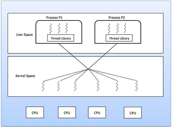
• Many to many relationship.
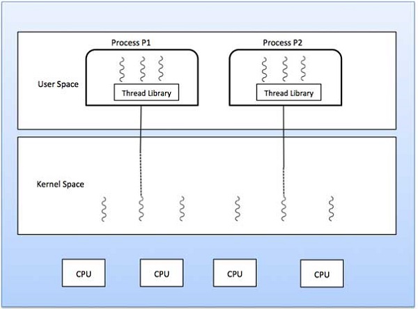
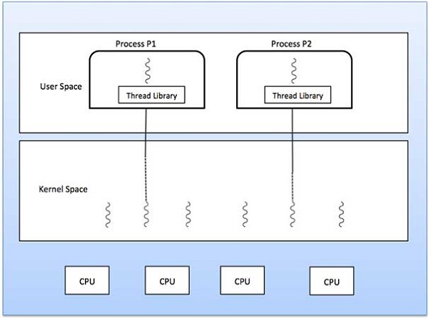
• Many to one relationship.
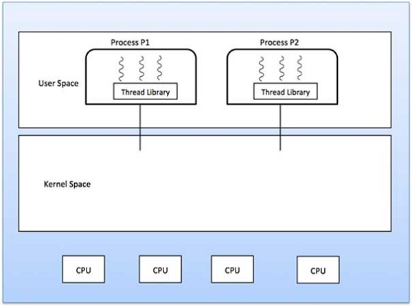
• One to one relationship.

Many to Many Model

The many-to-many model multiplexes any number of user threads onto an equal or smaller number of kernel threads.

The following diagram shows the many-to-many threading model where 6 user level threads are multiplexing with 6 kernel level threads. In this model, developers can create as many user threads as necessary and the corresponding Kernel threads can run in parallel on a multiprocessor machine. This model provides the best accuracy on concurrency and when a thread performs a blocking system call, the kernel can schedule another thread for execution.

Many to One Model

Many-to-one model maps many user level threads to one Kernel-level thread. Thread management is done in user space by the thread library. When thread makes a blocking system call, the entire process will be blocked. Only one thread can access the Kernel at a time, so multiple threads are unable to run in parallel on multiprocessors.

If the user-level thread libraries are implemented in the operating system in such a way that the system does not support them, then the Kernel threads use the many-to-one relationship modes.

One to One Model

There is one-to-one relationship of user-level thread to the kernel-level thread. This model provides more concurrency than the many-to-one model. It also allows another thread to run when a thread makes a blocking system call. It supports multiple threads to execute in parallel on microprocessors.

Disadvantage of this model is that creating user thread requires the corresponding Kernel thread. OS/2, windows NT and windows 2000 use one to one relationship model.

Difference between User-Level & Kernel-Level Thread

S.N.	User-Level Threads	Kernel-Level Thread
1	User-level threads are faster to create and manage.	Kernel-level threads are slower to create and manage.
2	Implementation is by a thread library at the user level.	Operating system supports creation of Kernel threads.
3	User-level thread is generic and can run on any operating system.	Kernel-level thread is specific to the operating system.
4	Multi-threaded applications cannot take advantage of multiprocessing.	Kernel routines themselves can be multithreaded.

Inter Process Communication (IPC)

A process can be of two type:

• Independent process.
• Co-operating process.

An independent process is not affected by the execution of other processes while a co-operating process can be affected by other executing processes. Though one can think that those processes, which are running independently, will execute very efficiently but in practical, there are many situations when co-operative nature can be utilised for increasing computational speed, convenience and modularity. Inter process communication (IPC) is a mechanism which allows processes to communicate each other and synchronize their actions. The communication between these processes can be seen as a method of co-operation between them. Processes can communicate with each other using these two ways:

1. Shared Memory
2. Message passing

The Figure 1 below shows a basic structure of communication between processes via shared memory method and via message passing.

An operating system can implement both method of communication. First, we will discuss the shared memory method of communication and then message passing. Communication between processes using shared memory requires processes to share some variable and it completely depends on how programmer will implement it. One way of communication using shared memory can be imagined like this: Suppose process1 and process2 are executing simultaneously and they share some resources or use some information from other process, process1 generate information about certain computations or resources being used and keeps it as a record in shared memory. When process2 need to use the shared information, it will check in the record stored in shared memory and take note of the information generated by process1 and act accordingly. Processes can use shared memory for extracting information as a record from other process as well as for delivering any specific information to other process.
Let’s discuss an example of communication between processes using shared memory method.

i) Shared Memory Method

Ex: Producer-Consumer problem
There are two processes: Producer and Consumer. Producer produces some item and Consumer consumes that item. The two processes shares a common space or memory location known as buffer where the item produced by Producer is stored and from where the Consumer consumes the item if needed. There are two version of this problem: first one is known as unbounded buffer problem in which Producer can keep on producing items and there is no limit on size of buffer, the second one is known as bounded buffer problem in which producer can produce up to a certain amount of item and after that it starts waiting for consumer to consume it. We will discuss the bounded buffer problem. First, the Producer and the Consumer will share some common memory, then producer will start producing items. If the total produced item is equal to the size of buffer, producer will wait to get it consumed by the Consumer. Sim-
ilarly, the consumer first check for the availability of the item and if no item is available, Consumer will wait for producer to produce it. If there are items available, consumer will consume it. The pseudo code are given below:
Shared Data between the two Processes

#define buff_max 25 #define mod %        struct item{            // different member of the produced data          // or consumed data             ---------     }            // An array is needed for holding the items.      // This is the shared place which will be       // access by both process        // item shared_buff [ buff_max ];             // Two variables which will keep track of      // the indexes of the items produced by producer      // and consumer The free index points to      // the next free index. The full index points to      // the first full index.      int free_index = 0;     int full_index = 0;

Producer Process Code

item nextProduced;            while(1){                    // check if there is no space          // for production.         // if so keep waiting.         while((free_index+1) mod buff_max == full_index);                    shared_buff[free_index] = nextProduced;         free_index = (free_index + 1) mod buff_max;     }

Consumer Process Code

item nextConsumed;            while(1){                    // check if there is an available          // item  for consumption.          // if not keep on waiting for          // get them produced.         while((free_index == full_index);                    nextConsumed = shared_buff[full_index];         full_index = (full_index + 1) mod buff_max;     }

In the above code, The producer will start producing again when the (free_index+1) mod buff max will be free because if it it not free, this implies that there are still items that can be consumed by the Consumer so there is no need to produce more. Similarly, if free index and full index points to the same index, this implies that there are no item to consume.

ii) Messaging Passing Method

Now, We will start our discussion for the communication between processes via message passing. In this method, processes communicate with each other without using any kind of shared memory. If two processes p1 and p2 want to communicate with each other, they proceed as follow:

• Establish a communication link (if a link already exists, no need to establish it again.)
• Start exchanging messages using basic primitives.
  We need at least two primitives:
  – send(message, destinaion) or send(message)
  – receive(message, host) or receive(message)

The message size can be of fixed size or of variable size. if it is of fixed size, it is easy for OS designer but complicated for programmer and if it is of variable size then it is easy for programmer but complicated for the OS designer. A standard message can have two parts: header and body.
The header part is used for storing Message type, destination id, source id, message length and control information. The control information contains information like what to do if runs out of buffer space, sequence number, priority. Generally, message is sent using FIFO style.

Message Passing through Communication Link.

Direct and Indirect Communication link
Now, We will start our discussion about the methods of implementing communication link. While implementing the link, there are some questions which need to be kept in mind like :

1. How are links established?
2. Can a link be associated with more than two processes?
3. How many links can there be between every pair of communicating processes?
4. What is the capacity of a link? Is the size of a message that the link can accommodate fixed or variable?
5. Is a link unidirectional or bi-directional?

A link has some capacity that determines the number of messages that can reside in it temporarily for which Every link has a queue associated with it which can be either of zero capacity or of bounded capacity or of unbounded capacity. In zero capacity, sender wait until receiver inform sender that it has received the message. In non-zero capacity cases, a process does not know whether a message has been received or not after the send operation. For this, the sender must communicate to receiver explicitly. Implementation of the link depends on the situation, it can be either a Direct communication link or an In-directed communication link.
Direct Communication links are implemented when the processes use specific process identifier for the communication but it is hard to identify the sender ahead of time.
For example: the print server.

In-directed Communication is done via a shred mailbox (port), which consists of queue of messages. Sender keeps the message in mailbox and receiver picks them up.

Message Passing through Exchanging the Messages.

Synchronous and Asynchronous Message Passing:
A process that is blocked is one that is waiting for some event, such as a resource becoming available or the completion of an I/O operation. IPC is possible between the processes on same computer as well as on the processes running on different computer i.e. in networked/distributed system. In both cases, the process may or may not be blocked while sending a message or attempting to receive a message so Message passing may be blocking or non-blocking. Blocking is considered synchronous and blocking send means the sender will be blocked until the message is received by receiver. Similarly, blocking receive has the receiver block until a message is available. Non-blocking is considered asynchronous and Non-blocking send has the sender sends the message and continue. Similarly, Non-blocking receive has the receiver receive a valid message or null. After a careful analysis, we can come to a conclusion that, for a sender it is more natural to be non-blocking after message passing as there may be a need to send the message to different processes But the sender expect acknowledgement from receiver in case the send fails. Similarly, it is more natural for a receiver to be blocking after issuing the receive as the information from the received message may be used for further execution but at the same time, if the message send keep on failing, receiver will have to wait for indefinitely. That is why we also consider the other possibility of message passing. There are basically three most preferred combinations:

• Blocking send and blocking receive
• Non-blocking send and Non-blocking receive
• Non-blocking send and Blocking receive (Mostly used)

In Direct message passing, The process which want to communicate must explicitly name the recipient or sender of communication.
e.g. send(p1, message) means send the message to p1.
similarly, receive(p2, message) means receive the message from p2.
In this method of communication, the communication link get established automatically, which can be either unidirectional or bidirectional, but one link can be used between one pair of the sender and receiver and one pair of sender and receiver should not possess more than one pair of link. Symmetry and asymmetry between the sending and receiving can also be implemented i.e. either both process will name each other for sending and receiving the messages or only sender will name receiver for sending the message and there is no need for receiver for naming the sender for receiving the message.The problem with this method of communication is that if the name of one process changes, this method will not work.

In Indirect message passing, processes uses mailboxes (also referred to as ports) for sending and receiving messages. Each mailbox has a unique id and processes can communicate only if they share a mailbox. Link established only if processes share a common mailbox and a single link can be associated with many processes. Each pair of processes can share several communication links and these link may be unidirectional or bi-directional. Suppose two process want to communicate though Indirect message passing, the required operations are: create a mail box, use this mail box for sending and receiving messages, destroy the mail box. The standard primitives used are : send(A, message) which means send the message to mailbox A. The primitive for the receiving the message also works in the same way e.g. received (A, message). There is a problem in this mailbox implementation. Suppose there are more than two processes sharing the same mailbox and suppose the process p1 sends a message to the mailbox, which process will be the receiver? This can be solved by either forcing that only two processes can share a single mailbox or enforcing that only one process is allowed to execute the receive at a given time or select any process randomly and notify the sender about the receiver. A mailbox can be made private to a single sender/receiver pair and can also be shared between multiple sender/receiver pairs. Port is an implementation of such mailbox which can have multiple sender and single receiver. It is used in client/server application (Here server is the receiver). The port is owned by the receiving process and created by OS on the request of the receiver process and can be destroyed either on request of the same receiver process or when the receiver terminates itself. Enforcing that only one process is allowed to execute the receive can be done using the concept of mutual exclusion. Mutex mailbox is create which is shared by n process. Sender is non-blocking and sends the message. The first process which executes the receive will enter in the critical section and all other processes will be blocking and will wait.

Now, lets discuss the Producer-Consumer problem using message passing concept. The producer place items (inside messages) in the mailbox and the consumer can consume item when at least one message present in the mailbox. The code are given below:

Producer Code

void Producer(void){                    int item;         Message m;                    while(1){                            receive(Consumer, &m);             item = produce();             build_message(&m , item ) ;             send(Consumer, &m);         }     }

Consumer Code

void Consumer(void){                    int item;         Message m;                    while(1){                            receive(Producer, &m);             item = extracted_item();             send(Producer, &m);             consume_item(item);         }     }

Examples of IPC systems

1. Posix : uses shared memory method.
2. Mach : uses message passing
3. Windows XP : uses message passing using local procedural calls

Communication in client/server Architecture:

There are various mechanism:

• Pipe
• Socket
• Remote Procedural calls (RPCs)

The above three methods will be discussed later article as all of them are quite conceptual and deserve their own separate articles.

Scheduling Criteria

• Different CPU scheduling algorithms has different properties. Selection decision depends on the properties of various algorithms.
• There are many criteria need to be consider for comparing CPU scheduling algorithms.
• This characteristic is used to determine the best algorithm. The criteria are as following:

1. CPU Utilization

• We want to keep the CPU as busy as possible. It may range from 0 to 100%. In real time system, it suits range from 40% (for a lightly loaded system ) to 90% ( for heavily loaded system ).

2. Throughput

• If the CPU is busy executing processes, then work is being done. One measure of work is the number of processes completed per time unit for throughput. For time processes, these may be a one process for one minute. For shorter transactions, throughput might be 10 processes per minute.

3. Turnaround Time

• From the submission time of a process to its completion time is turnaround time. It is the sum of total time period spends waiting to get into memory, waiting in the ready queue, executing in the CPU and doing input/output operations.

4. Waiting Time

• The CPU scheduling algorithm does not affect the amount of the time during which process execute or does input/output. It affects only the amount of time that a process spends waiting in the ready queue. Waiting time is the sum of period spends waiting in the ready queue.

5. Response Time

• In an interactive system, a process can produce some output early and can continue, computing new results. Previous results are being displayed the user. Thus another measure is the time from the submission to the request until the first response is produced. It is called Response time. The turnaround time is normally limited by speed of output device.

Scheduling Algorithm

A Process Scheduler schedules different processes to be assigned to the CPU based on particular scheduling algorithms. There are six popular process scheduling algorithms which we are going to discuss in this chapter −

• First-Come, First-Served (FCFS) Scheduling
• Shortest-Job-Next (SJN) Scheduling
• Priority Scheduling
• Shortest Remaining Time
• Round Robin(RR) Scheduling
• Multiple-Level Queues Scheduling

These algorithms are either non-preemptive or preemptive. Non-preemptive algorithms are designed so that once a process enters the running state, it cannot be preempted until it completes its allotted time, whereas the preemptive scheduling is based on priority where a scheduler may preempt a low priority running process anytime when a high priority process enters into a ready state.

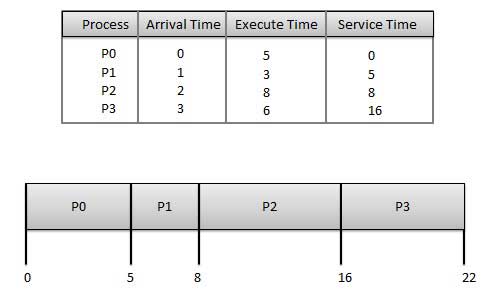
First Come First Serve (FCFS)

• Jobs are executed on first come, first serve basis.
• It is a non-preemptive, pre-emptive scheduling algorithm.
• Easy to understand and implement.
• Its implementation is based on FIFO queue.
• Poor in performance as average wait time is high.

Wait time of each process is as follows −

Process	Wait Time : Service Time - Arrival Time
P0	0 - 0 = 0
P1	5 - 1 = 4
P2	8 - 2 = 6
P3	16 - 3 = 13

Average Wait Time: (0+4+6+13) / 4 = 5.75

Shortest Job Next (SJN)

• This is also known as shortest job first, or SJF
• This is a non-preemptive, pre-emptive scheduling algorithm.
• Best approach to minimize waiting time.
• Easy to implement in Batch systems where required CPU time is known in advance.
• Impossible to implement in interactive systems where required CPU time is not known.
• The processer should know in advance how much time process will take.

Given: Table of processes, and their Arrival time, Execution time

Process	Arrival Time	Execution Time	Service Time
P0	0	5	0
P1	1	3	5
P2	2	8	14
P3	3	6	8

Waiting time of each process is as follows −

Process	Waiting Time
P0	0 - 0 = 0
P1	5 - 1 = 4
P2	14 - 2 = 12
P3	8 - 3 = 5

Average Wait Time: (0 + 4 + 12 + 5)/4 = 21 / 4 = 5.25

Priority Based Scheduling

• Priority scheduling is a non-preemptive algorithm and one of the most common scheduling algorithms in batch systems.
• Each process is assigned a priority. Process with highest priority is to be executed first and so on.
• Processes with same priority are executed on first come first served basis.
• Priority can be decided based on memory requirements, time requirements or any other resource requirement.

Given: Table of processes, and their Arrival time, Execution time, and priority. Here we are considering 1 is the lowest priority.

Process	Arrival Time	Execution Time	Priority	Service Time
P0	0	5	1	0
P1	1	3	2	11
P2	2	8	1	14
P3	3	6	3	5

Waiting time of each process is as follows −

Process	Waiting Time
P0	0 - 0 = 0
P1	11 - 1 = 10
P2	14 - 2 = 12
P3	5 - 3 = 2

Average Wait Time: (0 + 10 + 12 + 2)/4 = 24 / 4 = 6

Shortest Remaining Time

• Shortest remaining time (SRT) is the preemptive version of the SJN algorithm.
• The processor is allocated to the job closest to completion but it can be preempted by a newer ready job with shorter time to completion.
• Impossible to implement in interactive systems where required CPU time is not known.
• It is often used in batch environments where short jobs need to give preference.

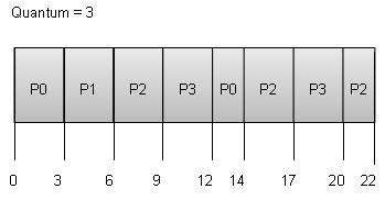
Round Robin Scheduling

• Round Robin is the preemptive process scheduling algorithm.
• Each process is provided a fix time to execute, it is called a quantum.
• Once a process is executed for a given time period, it is preempted and other process executes for a given time period.
• Context switching is used to save states of preempted processes.

Wait time of each process is as follows −

Process	Wait Time : Service Time - Arrival Time
P0	(0 - 0) + (12 - 3) = 9
P1	(3 - 1) = 2
P2	(6 - 2) + (14 - 9) + (20 - 17) = 12
P3	(9 - 3) + (17 - 12) = 11

Average Wait Time: (9+2+12+11) / 4 = 8.5

Multiple-Level Queues Scheduling

Multiple-level queues are not an independent scheduling algorithm. They make use of other existing algorithms to group and schedule jobs with common characteristics.

• Multiple queues are maintained for processes with common characteristics.
• Each queue can have its own scheduling algorithms.
• Priorities are assigned to each queue.

For example, CPU-bound jobs can be scheduled in one queue and all I/O-bound jobs in another queue. The Process Scheduler then alternately selects jobs from each queue and assigns them to the CPU based on the algorithm assigned to the queue.

Multiple-Processor Scheduling in Operating System

In multiple-processor scheduling multiple CPU’s are available and hence Load Sharing becomes possible. However multiple processor scheduling is more complex as compared to single processor scheduling. In multiple processor scheduling there are cases when the processors are identical i.e. HOMOGENEOUS, in terms of their functionality, we can use any processor available to run any process in the queue.

Approaches to Multiple-Processor Scheduling –

One approach is when all the scheduling decisions and I/O processing are handled by a single processor which is called the Master Server and the other processors executes only the user code. This is simple and reduces the need of data sharing. This entire scenario is called Asymmetric Multiprocessing.

A second approach uses Symmetric Multiprocessing where each processor is self scheduling. All processes may be in a common ready queue or each processor may have its own private queue for ready processes. The scheduling proceeds further by having the scheduler for each processor examine the ready queue and select a process to execute.

Processor Affinity –

Processor Affinity means a processes has an affinity for the processor on which it is currently running.
When a process runs on a specific processor there are certain effects on the cache memory. The data most recently accessed by the process populate the cache for the processor and as a result successive memory access by the process are often satisfied in the cache memory. Now if the process migrates to another processor, the contents of the cache memory must be invalidated for the first processor and the cache for the second processor must be repopulated. Because of the high cost of invalidating and repopulating caches, most of the SMP(symmetric multiprocessing) systems try to avoid migration of processes from one processor to another and try to keep a process running on the same processor. This is known as PROCESSOR AFFINITY.

There are two types of processor affinity:

1. Soft Affinity – When an operating system has a policy of attempting to keep a process running on the same processor but not guaranteeing it will do so, this situation is called soft affinity.
2. Hard Affinity – Some systems such as Linux also provide some system calls that support Hard Affinity which allows a process to migrate between processors.

Load Balancing –

Load Balancing is the phenomena which keeps the workload evenly distributed across all processors in an SMP system. Load balancing is necessary only on systems where each processor has its own private queue of process which are eligible to execute. Load balancing is unnecessary because once a processor becomes idle it immediately extracts a runnable process from the common run queue. On SMP(symmetric multiprocessing), it is important to keep the workload balanced among all processors to fully utilize the benefits of having more than one processor else one or more processor will sit idle while other processors have high workloads along with lists of processors awaiting the CPU.

There are two general approaches to load balancing :

1. Push Migration – In push migration a task routinely checks the load on each processor and if it finds an imbalance then it evenly distributes load on each processors by moving the processes from overloaded to idle or less busy processors.
2. Pull Migration – Pull Migration occurs when an idle processor pulls a waiting task from a busy processor for its execution.

Multicore Processors –

In multicore processors multiple processor cores are places on the same physical chip. Each core has a register set to maintain its architectural state and thus appears to the operating system as a separate physical processor. SMP systems that use multicore processors are faster and consume less power than systems in which each processor has its own physical chip.

However multicore processors may complicate the scheduling problems. When processor accesses memory then it spends a significant amount of time waiting for the data to become available. This situation is called MEMORY STALL. It occurs for various reasons such as cache miss, which is accessing the data that is not in the cache memory. In such cases the processor can spend upto fifty percent of its time waiting for data to become available from the memory. To solve this problem recent hardware designs have implemented multithreaded processor cores in which two or more hardware threads are assigned to each core. Therefore if one thread stalls while waiting for the memory, core can switch to another thread.

There are two ways to multithread a processor :

1. Coarse-Grained Multithreading – In coarse grained multithreading a thread executes on a processor until a long latency event such as a memory stall occurs, because of the delay caused by the long latency event, the processor must switch to another thread to begin execution. The cost of switching between threads is high as the instruction pipeline must be terminated before the other thread can begin execution on the processor core. Once this new thread begins execution it begins filling the pipeline with its instructions.
2. Fine-Grained Multithreading – This multithreading switches between threads at a much finer level mainly at the boundary of an instruction cycle. The architectural design of fine grained systems include logic for thread switching and as a result the cost of switching between threads is small.

Virtualization and Threading –

In this type of multiple-processor scheduling even a single CPU system acts like a multiple-processor system. In a system with Virtualization, the virtualization presents one or more virtual CPU to each of virtual machines running on the system and then schedules the use of physical CPU among the virtual machines. Most virtualized environments have one host operating system and many guest operating systems. The host operating system creates and manages the virtual machines. Each virtual machine has a guest operating system installed and applications run within that guest.Each guest operating system may be assigned for specific use cases,applications or users including time sharing or even real-time operation. Any guest operating-system scheduling algorithm that assumes a certain amount of progress in a given amount of time will be negatively impacted by the virtualization. A time sharing operating system tries to allot 100 milliseconds to each time slice to give users a reasonable response time. A given 100 millisecond time slice may take much more than 100 milliseconds of virtual CPU time. Depending on how busy the system is, the time slice may take a second or more which results in a very poor response time for users logged into that virtual machine. The net effect of such scheduling layering is that individual virtualized operating systems receive only a portion of the available CPU cycles, even though they believe they are receiving all cycles and that they are scheduling all of those cycles.Commonly, the time-of-day clocks in virtual machines are incorrect because timers take no longer to trigger than they would on dedicated CPU’s.

Virtualizations can thus undo the good scheduling-algorithm efforts of the operating systems within virtual machines.

Real Time Scheduling

Priority based scheduling enables us to give better service to certain processes. In our discussion of multi-queue scheduling, priority was adjusted based on whether a task was more interactive or compute intensive. But most schedulers enable us to give any process any desired priority. Isn't that good enough?

Priority scheduling is inherently a best effort approach. If our task is competing with other high priority tasks, it may not get as much time as it requires. Sometimes best effort isn't good enough:

• During reentry, the space shuttle is aerodynamically unstable. It is not actually being kept under control by the quick reflexes of the well-trained pilots, but rather by guidance computers that are collecting attitude and acceleration input and adjusting numerous spoilers hundreds of times per second.
• Scientific and military satellites may receive precious and irreplaceable sensor data at extremely high speeds. If it takes us too long to receive, process, and store one data frame, the next data frame may be lost.
• More mundanely, but also important, many manufacturing processes are run by computers nowadays. An assembly line needs to move at a particular speed, with each step being performed at a particular time. Performing the action too late results in a flawed or useless product.
• Even more commonly, playing media, like video or audio, has real time requirements. Sound must be produced at a certain rate and frames must be displayed frequently enough or the media becomes uncomfortable to deal with.

There are many computer controlled applications where delays in critical processing can have undesirable, or even disastrous consequences.

What are Real-Time Systems

A real-time system is one whose correctness depends on timing as well as functionality.

When we discussed more traditional scheduling algorithms, the metrics we looked at were turn-around time (or throughput), fairness, and mean response time. But real-time systems have very different requirements, characterized by different metrics:

• timeliness ... how closely does it meet its timing requirements (e.g. ms/day of accumulated tardiness)
• predictability ... how much deviation is there in delivered timeliness

And we introduce a few new concepts:

• feasibility ... whether or not it is possible to meet the requirements for a particular task set
• hard real-time ... there are strong requirements that specified tasks be run a specified intervals (or within a specified response time). Failure to meet this requirement (perhaps by as little as a fraction of a micro-second) may result in system failure.
• soft real-time ... we may want to provide very good (e.g. microseconds) response time, the only consequences of missing a deadline are degraded performance or recoverable failures.

It sounds like real-time scheduling is more critical and difficult than traditional time-sharing, and in many ways it is. But real-time systems may have a few characteristics that make scheduling easier:

• We may actually know how long each task will take to run. This enables much more intelligent scheduling.
• Starvation (of low priority tasks) may be acceptable. The space shuttle absolutely must sense attitude and acceleration and adjust spolier positions once per millisecond. But it probably doesn't matter if we update the navigational display once per millisecond or once every ten seconds. Telemetry transmission is probably somewhere in-between. Understanding the relative criticality of each task gives us the freedom to intelligently shed less critical work in times of high demand.
• The work-load may be relatively fixed. Normally high utilization implies long queuing delays, as bursty traffic creates long lines. But if the incoming traffic rate is relatively constant, it is possible to simultaneously achieve high utilization and good response time.

Real-Time Scheduling Algorithms

In the simplest real-time systems, where the tasks and their execution times are all known, there might not even be a scheduler. One task might simply call (or yield to) the next. This model makes a great deal of sense in a system where the tasks form a producer/consumer pipeline (e.g. MPEG frame receipt, protocol decoding, image decompression, display).

In more complex real-time system, with a larger (but still fixed) number of tasks that do not function in a strictly pipeline fashion, it may be possible to do static scheduling. Based on the list of tasks to be run, and the expected completion time for each, we can define (at design or build time) a fixed schedule that will ensure timely execution of all tasks.

But for many real-time systems, the work-load changes from moment to moment, based on external events. These require dynamic scheduling. For dynamic scheduling algorithms, there are two key questions:

1. how they choose the next (ready) task to run
   • shortest job first
   • static priority ... highest priority ready task
   • soonest start-time deadline first (ASAP)
   • soonest completion-time deadline first (slack time)
2. how they handle overload (infeasible requirements)
   • best effort
   • periodicity adjustments ... run lower priority tasks less often.
   • work shedding ... stop running lower priority tasks entirely.

Preemption may also be a different issue in real-time systems. In ordinary time-sharing, preemption is a means of improving mean response time by breaking up the execution of long-running, compute-intensive tasks. A second advantage of preemptive scheduling, particularly important in a general purpose timesharing system, is that it prevents a buggy (infinite loop) program from taking over the CPU. The trade-off, between improved response time and increased overhead (for the added context switches), almost always favors preemptive scheduling. This may not be true for real-time systems:

• preempting a running task will almost surely cause it to miss its completion deadline.
• since we so often know what the expected execution time for a task will be, we can schedule accordingly and should have little need for preemption.
• embedded and real-time systems run fewer and simpler tasks than general purpose time systems, and the code is often much better tested ... so infinite loop bugs are extremely rare.

For the least demanding real time tasks, a sufficiently lightly loaded system might be reasonably successful in meeting its deadlines. However, this is achieved simply because the frequency at which the task is run happens to be high enough to meet its real time requirements, not because the scheduler is aware of such requirements. A lightly loaded machine running a traditional scheduler can often display a video to a user's satisfaction, not because the scheduler "knows" that a frame must be rendered by a certain deadline, but simply because the machine has enough cycles and a low enough work load to render the frame before the deadline has arrived.


Thank you,
By Er. Shejwal Shrikant.
31-12-2019, Tuesday.