Greedy Algorithm
Greedy Algorithm
Introduction to Greedy technique
Components of Greedy Algorithm
Greedy algorithms have the following five components −
1. A candidate set − A solution is created from this set.
2. A selection function − Used to choose the best candidate to be added to the solution.
3. A feasibility function − Used to determine whether a candidate can be used to contribute to the solution.
4. An objective function − Used to assign a value to a solution or a partial solution.
5. A solution function − Used to indicate whether a complete solution has been reached.
Optimal Merge Pattern
Let us consider the given files, f1, f2, f3, f4 and f5 with 20, 30, 10, 5 and 30 number of elements respectively.


Activity Selection Problem
Greedy is an algorithmic paradigm that builds up a solution piece by piece, always choosing the next piece that offers the most obvious and immediate benefit. Greedy algorithms are used for optimization problems. An optimization problem can be solved using Greedy if the problem has the following property: At every step, we can make a choice that looks best at the moment, and we get the optimal solution of the complete problem.
If a Greedy Algorithm can solve a problem, then it generally becomes the best method to solve that problem as the Greedy algorithms are in general more efficient than other techniques like Dynamic Programming. But Greedy algorithms cannot always be applied. For example, Fractional Knapsack problem (See this) can be solved using Greedy, but 0-1 Knapsack cannot be solved using Greedy.
Following are some standard algorithms that are Greedy algorithms.
1) Kruskal’s Minimum Spanning Tree (MST): In Kruskal’s algorithm, we create a MST by picking edges one by one. The Greedy Choice is to pick the smallest weight edge that doesn’t cause a cycle in the MST constructed so far.
2) Prim’s Minimum Spanning Tree: In Prim’s algorithm also, we create a MST by picking edges one by one. We maintain two sets: a set of the vertices already included in MST and the set of the vertices not yet included. The Greedy Choice is to pick the smallest weight edge that connects the two sets.
3) Dijkstra’s Shortest Path: The Dijkstra’s algorithm is very similar to Prim’s algorithm. The shortest path tree is built up, edge by edge. We maintain two sets: a set of the vertices already included in the tree and the set of the vertices not yet included. The Greedy Choice is to pick the edge that connects the two sets and is on the smallest weight path from source to the set that contains not yet included vertices.
4) Huffman Coding: Huffman Coding is a loss-less compression technique. It assigns variable-length bit codes to different characters. The Greedy Choice is to assign least bit length code to the most frequent character.
The greedy algorithms are sometimes also used to get an approximation for Hard optimization problems. For example, Traveling Salesman Problem is a NP-Hard problem. A Greedy choice for this problem is to pick the nearest unvisited city from the current city at every step. This solutions don’t always produce the best optimal solution but can be used to get an approximately optimal solution.
Letus consider the Activity Selection problem as our first example of Greedy algorithms. Following is the problem statement.
You are given n activities with their start and finish times. Select the maximum number of activities that can be performed by a single person, assuming that a person can only work on a single activity at a time.
Example 1 : Consider the following 3 activities sorted by by finish time.
start[] = {10, 12, 20};
finish[] = {20, 25, 30};
A person can perform at most two activities. The maximum set of activities that can be executed is {0, 2} [ These are indexes in start[] and finish[] ]
Example 2 : Consider the following 6 activities sorted by by finish time.
start[] = {1, 3, 0, 5, 8, 5};
finish[] = {2, 4, 6, 7, 9, 9};
A person can perform at most four activities. The maximum set of activities that can be executed is {0, 1, 3, 4} [ These are indexes in start[] and finish[] ]
Huffman Coding
Prefix Codes, means the codes (bit sequences) are assigned in such a way that the code assigned to one character is not the prefix of code assigned to any other character. This is how Huffman Coding makes sure that there is no ambiguity when decoding the generated bitstream.
Let us understand prefix codes with a counter example. Let there be four characters a, b, c and d, and their corresponding variable length codes be 00, 01, 0 and 1. This coding leads to ambiguity because code assigned to c is the prefix of codes assigned to a and b. If the compressed bit stream is 0001, the de-compressed output may be “cccd” or “ccb” or “acd” or “ab”.
See this for applications of Huffman Coding.
There are mainly two major parts in Huffman Coding
1) Build a Huffman Tree from input characters.
2) Traverse the Huffman Tree and assign codes to characters.
Steps to build Huffman Tree
Input is an array of unique characters along with their frequency of occurrences and output is Huffman Tree.
1. Create a leaf node for each unique character and build a min heap of all leaf nodes (Min Heap is used as a priority queue. The value of frequency field is used to compare two nodes in min heap. Initially, the least frequent character is at root)
2. Extract two nodes with the minimum frequency from the min heap.
3. Create a new internal node with a frequency equal to the sum of the two nodes frequencies. Make the first extracted node as its left child and the other extracted node as its right child. Add this node to the min heap.
4. Repeat steps#2 and #3 until the heap contains only one node. The remaining node is the root node and the tree is complete.
Let us understand the algorithm with an example:
character Frequency
a 5
b 9
c 12
d 13
e 16
f 45
Step 1. Build a min heap that contains 6 nodes where each node represents root of a tree with single node.
Step 2 :Extract two minimum frequency nodes from min heap. Add a new internal node with frequency 5 + 9 = 14.

Now min heap contains 5 nodes where 4 nodes are roots of trees with single element each, and one heap node is root of tree with 3 elements
character Frequency
c 12
d 13
Internal Node 14
e 16
f 45
Step 3: Extract two minimum frequency nodes from heap. Add a new internal node with frequency 12 + 13 = 25

 Now min heap contains 4 nodes where 2 nodes are roots of trees with single element each, and two heap nodes are root of tree with more than one nodes.
character Frequency
Internal Node 14
e 16
Internal Node 25
f 45
Step 4: Extract two minimum frequency nodes. Add a new internal node with frequency 14 + 16 = 30

 Now min heap contains 3 nodes.
character Frequency Internal Node 25 Internal Node 30 f 45
Step 5: Extract two minimum frequency nodes. Add a new internal node with frequency 25 + 30 = 55

 Now min heap contains 2 nodes.
character Frequency
f 45
Internal Node 55
Step 6: Extract two minimum frequency nodes. Add a new internal node with frequency 45 + 55 = 100

 Now min heap contains only one node.
character Frequency Internal Node 100
Since the heap contains only one node, the algorithm stops here.
Steps to print codes from Huffman Tree:
Traverse the tree formed starting from the root. Maintain an auxiliary array. While moving to the left child, write 0 to the array. While moving to the right child, write 1 to the array. Print the array when a leaf node is encountered.

The codes are as follows:
character code-word
f. 0
c 100
d 101
a 1100
b 1101
e 111
Job Sequencing with Deadline
Given an array of jobs where every job has a deadline and associated profit if the job is finished before the deadline. It is also given that every job takes single unit of time, so the minimum possible deadline for any job is 1. How to maximize total profit if only one job can be scheduled at a time.
Examples:

This is a standard Greedy Algorithm problem. Following is algorithm.
1) Sort all jobs in decreasing order of profit.
2) Initialize the result sequence as first job in sorted jobs.
3) Do following for remaining n-1 jobs
…….a) If the current job can fit in the current result sequence without missing the deadline, add current job to the result. Else ignore the current job.
The costly operation in the Greedy solution is to assign a free slot for a job. We were traversing each and every slot for a job and assigning the greatest possible time slot(<deadline) which was available.
Suppose that a job J1 has a deadline of time t = 5. We assign the greatest time slot which is free and less than the deadline i.e 4-5 for this job. Now another job J2 with deadline of 5 comes in, so the time slot allotted will be 3-4 since 4-5 has already been allotted to job J1.
Now we assign the greatest possible time slot since if we assign a time slot even lesser than the available one than there might be some other job which will miss its deadline.
Example:
J1 with deadline d1 = 5, profit 40
J2 with deadline d2 = 1, profit 20
Suppose that for job J1 we assigned time slot of 0-1. Now job J2 cannot be performed since we will perform Job J1 during that time slot.
All time slots are individual sets initially. We first find the maximum deadline of all jobs. Let the max deadline be m. We create m+1 individual sets. If a job is assigned a time slot of t where t => 0, then the job is scheduled during [t-1, t]. So a set with value X represents the time slot [X-1, X].
We need to keep track of the greatest time slot available which can be allotted to a given job having deadline. We use the parent array of Disjoint Set Data structures for this purpose. The root of the tree is always the latest available slot. If for a deadline d, there is no slot available, then root would be 0.
A Minimum Spanning Tree (MST) is a subset of edges of a connected weighted undirected graph that connects all the vertices together with the minimum possible total edge weight. To derive an MST, Prim’s algorithm or Kruskal’s algorithm can be used. Hence, we will discuss Prim’s algorithm in this chapter.

Prim’s algorithm is a greedy approach to find the minimum spanning tree. In this algorithm, to form a MST we can start from an arbitrary vertex.
Using Prim’s algorithm, we can start from any vertex, let us start from vertex 1.

Dijkstra’s algorithm solves the single-source shortest-paths problem on a directed weighted graph G = (V, E), where all the edges are non-negative (i.e., w(u, v) ≥ 0 for each edge (u, v) Є E).
The complexity of this algorithm is fully dependent on the implementation of Extract-Min function. If extract min function is implemented using linear search, the complexity of this algorithm is O(V2 + E).
Let us consider vertex 1 and 9 as the start and destination vertex respectively. Initially, all the vertices except the start vertex are marked by ∞ and the start vertex is marked by 0.


Introduction to Greedy technique
Among all the algorithmic approaches, the simplest and straightforward approach is the Greedy method. In this approach, the decision is taken on the basis of current available information without worrying about the effect of the current decision in future.
Greedy algorithms build a solution part by part, choosing the next part in such a way, that it gives an immediate benefit. This approach never reconsiders the choices taken previously. This approach is mainly used to solve optimization problems. Greedy method is easy to implement and quite efficient in most of the cases. Hence, we can say that Greedy algorithm is an algorithmic paradigm based on heuristic that follows local optimal choice at each step with the hope of finding global optimal solution.
In many problems, it does not produce an optimal solution though it gives an approximate (near optimal) solution in a reasonable time.
Example
Example
Example:
- machine scheduling
- Fractional Knapsack Problem
- Minimum Spanning Tree
- Huffman Code
- Job Sequencing
- Activity Selection Problem
Components of Greedy Algorithm
Greedy algorithms have the following five components −
1. A candidate set − A solution is created from this set.
2. A selection function − Used to choose the best candidate to be added to the solution.
3. A feasibility function − Used to determine whether a candidate can be used to contribute to the solution.
4. An objective function − Used to assign a value to a solution or a partial solution.
5. A solution function − Used to indicate whether a complete solution has been reached.
Optimal Merge Pattern
Merge a set of sorted files of different length into a single sorted file. We need to find an optimal solution, where the resultant file will be generated in minimum time.
If the number of sorted files are given, there are many ways to merge them into a single sorted file. This merge can be performed pair wise. Hence, this type of merging is called as 2-way merge patterns.
As, different pairings require different amounts of time, in this strategy we want to determine an optimal way of merging many files together. At each step, two shortest sequences are merged.
To merge a p-record file and a q-record file requires possibly p + q record moves, the obvious choice being, merge the two smallest files together at each step.
Two-way merge patterns can be represented by binary merge trees. Let us consider a set of n sorted files {f1, f2, f3, …, fn}. Initially, each element of this is considered as a single node binary tree. To find this optimal solution, the following algorithm is used.
Algorithm: TREE (n)
for i := 1 to n – 1 do
declare new node
node.leftchild := least (list)
node.rightchild := least (list)
node.weight) := ((node.leftchild).weight) + ((node.rightchild).weight)
insert (list, node);
return least (list);
for i := 1 to n – 1 do
declare new node
node.leftchild := least (list)
node.rightchild := least (list)
node.weight) := ((node.leftchild).weight) + ((node.rightchild).weight)
insert (list, node);
return least (list);
At the end of this algorithm, the weight of the root node represents the optimal cost.
Example
Let us consider the given files, f1, f2, f3, f4 and f5 with 20, 30, 10, 5 and 30 number of elements respectively.
If merge operations are performed according to the provided sequence, then
M1 = merge f1 and f2 => 20 + 30 = 50
M2 = merge M1 and f3 => 50 + 10 = 60
M3 = merge M2 and f4 => 60 + 5 = 65
M4 = merge M3 and f5 => 65 + 30 = 95
Hence, the total number of operations is
50 + 60 + 65 + 95 = 270
Now, the question arises is there any better solution?
Sorting the numbers according to their size in an ascending order, we get the following sequence −
f4, f3, f1, f2, f5
Hence, merge operations can be performed on this sequence
M1 = merge f4 and f3 => 5 + 10 = 15
M2 = merge M1 and f1 => 15 + 20 = 35
M3 = merge M2 and f2 => 35 + 30 = 65
M4 = merge M3 and f5 => 65 + 30 = 95
Therefore, the total number of operations is
15 + 35 + 65 + 95 = 210
Obviously, this is better than the previous one.
In this context, we are now going to solve the problem using this algorithm.
Initial Set

Step-1
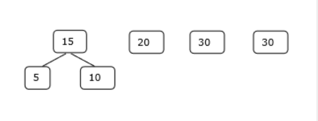
Step-2

Step-3

Step-4

Hence, the solution takes 15 + 35 + 60 + 95 = 205 number of comparisons.
Activity Selection Problem
Greedy is an algorithmic paradigm that builds up a solution piece by piece, always choosing the next piece that offers the most obvious and immediate benefit. Greedy algorithms are used for optimization problems. An optimization problem can be solved using Greedy if the problem has the following property: At every step, we can make a choice that looks best at the moment, and we get the optimal solution of the complete problem.
If a Greedy Algorithm can solve a problem, then it generally becomes the best method to solve that problem as the Greedy algorithms are in general more efficient than other techniques like Dynamic Programming. But Greedy algorithms cannot always be applied. For example, Fractional Knapsack problem (See this) can be solved using Greedy, but 0-1 Knapsack cannot be solved using Greedy.
Following are some standard algorithms that are Greedy algorithms.
1) Kruskal’s Minimum Spanning Tree (MST): In Kruskal’s algorithm, we create a MST by picking edges one by one. The Greedy Choice is to pick the smallest weight edge that doesn’t cause a cycle in the MST constructed so far.
2) Prim’s Minimum Spanning Tree: In Prim’s algorithm also, we create a MST by picking edges one by one. We maintain two sets: a set of the vertices already included in MST and the set of the vertices not yet included. The Greedy Choice is to pick the smallest weight edge that connects the two sets.
3) Dijkstra’s Shortest Path: The Dijkstra’s algorithm is very similar to Prim’s algorithm. The shortest path tree is built up, edge by edge. We maintain two sets: a set of the vertices already included in the tree and the set of the vertices not yet included. The Greedy Choice is to pick the edge that connects the two sets and is on the smallest weight path from source to the set that contains not yet included vertices.
4) Huffman Coding: Huffman Coding is a loss-less compression technique. It assigns variable-length bit codes to different characters. The Greedy Choice is to assign least bit length code to the most frequent character.
The greedy algorithms are sometimes also used to get an approximation for Hard optimization problems. For example, Traveling Salesman Problem is a NP-Hard problem. A Greedy choice for this problem is to pick the nearest unvisited city from the current city at every step. This solutions don’t always produce the best optimal solution but can be used to get an approximately optimal solution.
Letus consider the Activity Selection problem as our first example of Greedy algorithms. Following is the problem statement.
You are given n activities with their start and finish times. Select the maximum number of activities that can be performed by a single person, assuming that a person can only work on a single activity at a time.
Example 1 : Consider the following 3 activities sorted by by finish time.
start[] = {10, 12, 20};
finish[] = {20, 25, 30};
A person can perform at most two activities. The maximum set of activities that can be executed is {0, 2} [ These are indexes in start[] and finish[] ]
Example 2 : Consider the following 6 activities sorted by by finish time.
start[] = {1, 3, 0, 5, 8, 5};
finish[] = {2, 4, 6, 7, 9, 9};
A person can perform at most four activities. The maximum set of activities that can be executed is {0, 1, 3, 4} [ These are indexes in start[] and finish[] ]
Huffman Coding
Prefix Codes, means the codes (bit sequences) are assigned in such a way that the code assigned to one character is not the prefix of code assigned to any other character. This is how Huffman Coding makes sure that there is no ambiguity when decoding the generated bitstream.
Let us understand prefix codes with a counter example. Let there be four characters a, b, c and d, and their corresponding variable length codes be 00, 01, 0 and 1. This coding leads to ambiguity because code assigned to c is the prefix of codes assigned to a and b. If the compressed bit stream is 0001, the de-compressed output may be “cccd” or “ccb” or “acd” or “ab”.
See this for applications of Huffman Coding.
There are mainly two major parts in Huffman Coding
1) Build a Huffman Tree from input characters.
2) Traverse the Huffman Tree and assign codes to characters.
Steps to build Huffman Tree
Input is an array of unique characters along with their frequency of occurrences and output is Huffman Tree.
1. Create a leaf node for each unique character and build a min heap of all leaf nodes (Min Heap is used as a priority queue. The value of frequency field is used to compare two nodes in min heap. Initially, the least frequent character is at root)
2. Extract two nodes with the minimum frequency from the min heap.
3. Create a new internal node with a frequency equal to the sum of the two nodes frequencies. Make the first extracted node as its left child and the other extracted node as its right child. Add this node to the min heap.
4. Repeat steps#2 and #3 until the heap contains only one node. The remaining node is the root node and the tree is complete.
Let us understand the algorithm with an example:
character Frequency
a 5
b 9
c 12
d 13
e 16
f 45
Step 1. Build a min heap that contains 6 nodes where each node represents root of a tree with single node.
Step 2 :Extract two minimum frequency nodes from min heap. Add a new internal node with frequency 5 + 9 = 14.

Now min heap contains 5 nodes where 4 nodes are roots of trees with single element each, and one heap node is root of tree with 3 elements
character Frequency
c 12
d 13
Internal Node 14
e 16
f 45
Step 3: Extract two minimum frequency nodes from heap. Add a new internal node with frequency 12 + 13 = 25


character Frequency
Internal Node 14
e 16
Internal Node 25
f 45
Step 4: Extract two minimum frequency nodes. Add a new internal node with frequency 14 + 16 = 30


character Frequency Internal Node 25 Internal Node 30 f 45
Step 5: Extract two minimum frequency nodes. Add a new internal node with frequency 25 + 30 = 55


character Frequency
f 45
Internal Node 55
Step 6: Extract two minimum frequency nodes. Add a new internal node with frequency 45 + 55 = 100


character Frequency Internal Node 100
Since the heap contains only one node, the algorithm stops here.
Steps to print codes from Huffman Tree:
Traverse the tree formed starting from the root. Maintain an auxiliary array. While moving to the left child, write 0 to the array. While moving to the right child, write 1 to the array. Print the array when a leaf node is encountered.

The codes are as follows:
character code-word
f. 0
c 100
d 101
a 1100
b 1101
e 111
Job Sequencing with Deadline
Given an array of jobs where every job has a deadline and associated profit if the job is finished before the deadline. It is also given that every job takes single unit of time, so the minimum possible deadline for any job is 1. How to maximize total profit if only one job can be scheduled at a time.
Examples:

This is a standard Greedy Algorithm problem. Following is algorithm.
1) Sort all jobs in decreasing order of profit.
2) Initialize the result sequence as first job in sorted jobs.
3) Do following for remaining n-1 jobs
…….a) If the current job can fit in the current result sequence without missing the deadline, add current job to the result. Else ignore the current job.
Job Sequencing Problem Using Disjoint Set
Given a set of n jobs where each job i has a deadline di >=1 and profit pi>=0. Only one job can be scheduled at a time. Each job takes 1 unit of time to complete. We earn the profit if and only if the job is completed by its deadline. The task is to find the subset of jobs that maximizes profit.
Examples:
Input: Four Jobs with following deadlines and profits
JobID Deadline Profit
a 4 20
b 1 10
c 1 40
d 1 30
Output: Following is maximum profit sequence of jobs:
c, a
JobID Deadline Profit
a 4 20
b 1 10
c 1 40
d 1 30
Output: Following is maximum profit sequence of jobs:
c, a
Input: Five Jobs with following deadlines and profits
JobID Deadline Profit
a 2 100
b 1 19
c 2 27
d 1 25
e 3 15
Output: Following is maximum profit sequence of jobs:
c, a, e
JobID Deadline Profit
a 2 100
b 1 19
c 2 27
d 1 25
e 3 15
Output: Following is maximum profit sequence of jobs:
c, a, e
A greedy solution of time complexity O(n2) is already discussed here. Below is the simple Greedy Algorithm.
1. Sort all jobs in decreasing order of profit.
2. Initialize the result sequence as first job in sorted jobs.
3. Do following for remaining n-1 jobs
4. If the current job can fit in the current result sequence without missing the deadline, add current job to the result. Else ignore the current job.
The costly operation in the Greedy solution is to assign a free slot for a job. We were traversing each and every slot for a job and assigning the greatest possible time slot(<deadline) which was available.
What does greatest time slot means?
Suppose that a job J1 has a deadline of time t = 5. We assign the greatest time slot which is free and less than the deadline i.e 4-5 for this job. Now another job J2 with deadline of 5 comes in, so the time slot allotted will be 3-4 since 4-5 has already been allotted to job J1.
Why to assign greatest time slot(free) to a job?
Now we assign the greatest possible time slot since if we assign a time slot even lesser than the available one than there might be some other job which will miss its deadline.
Example:
J1 with deadline d1 = 5, profit 40
J2 with deadline d2 = 1, profit 20
Suppose that for job J1 we assigned time slot of 0-1. Now job J2 cannot be performed since we will perform Job J1 during that time slot.
Using Disjoint Set for Job Sequencing
All time slots are individual sets initially. We first find the maximum deadline of all jobs. Let the max deadline be m. We create m+1 individual sets. If a job is assigned a time slot of t where t => 0, then the job is scheduled during [t-1, t]. So a set with value X represents the time slot [X-1, X].
We need to keep track of the greatest time slot available which can be allotted to a given job having deadline. We use the parent array of Disjoint Set Data structures for this purpose. The root of the tree is always the latest available slot. If for a deadline d, there is no slot available, then root would be 0.
Minimum Spanning Tree
A Minimum Spanning Tree (MST) is a subset of edges of a connected weighted undirected graph that connects all the vertices together with the minimum possible total edge weight. To derive an MST, Prim’s algorithm or Kruskal’s algorithm can be used. Hence, we will discuss Prim’s algorithm in this chapter.
As we have discussed, one graph may have more than one spanning tree. If there are n number of vertices, the spanning tree should have n - 1 number of edges. In this context, if each edge of the graph is associated with a weight and there exists more than one spanning tree, we need to find the minimum spanning tree of the graph.
Moreover, if there exist any duplicate weighted edges, the graph may have multiple minimum spanning tree.

In the above graph, we have shown a spanning tree though it’s not the minimum spanning tree. The cost of this spanning tree is (5 + 7 + 3 + 3 + 5 + 8 + 3 + 4) = 38.
We will use Prim’s algorithm to find the minimum spanning tree.
1.Prim’s Algorithm
Prim’s algorithm is a greedy approach to find the minimum spanning tree. In this algorithm, to form a MST we can start from an arbitrary vertex.
Example
Using Prim’s algorithm, we can start from any vertex, let us start from vertex 1.
Vertex 3 is connected to vertex 1 with minimum edge cost, hence edge (1, 2) is added to the spanning tree.
Next, edge (2, 3) is considered as this is the minimum among edges {(1, 2), (2, 3), (3, 4), (3, 7)}.
In the next step, we get edge (3, 4) and (2, 4) with minimum cost. Edge (3, 4) is selected at random.
In a similar way, edges (4, 5), (5, 7), (7, 8), (6, 8) and (6, 9) are selected. As all the vertices are visited, now the algorithm stops.
The cost of the spanning tree is (2 + 2 + 3 + 2 + 5 + 2 + 3 + 4) = 23. There is no more spanning tree in this graph with cost less than 23.


2. Dijkstra’s Algorithm
Dijkstra’s algorithm solves the single-source shortest-paths problem on a directed weighted graph G = (V, E), where all the edges are non-negative (i.e., w(u, v) ≥ 0 for each edge (u, v) Є E).
In the following algorithm, we will use one function Extract-Min(), which extracts the node with the smallest key.
Analysis
The complexity of this algorithm is fully dependent on the implementation of Extract-Min function. If extract min function is implemented using linear search, the complexity of this algorithm is O(V2 + E).
In this algorithm, if we use min-heap on which Extract-Min() function works to return the node from Q with the smallest key, the complexity of this algorithm can be reduced further.
Example
Let us consider vertex 1 and 9 as the start and destination vertex respectively. Initially, all the vertices except the start vertex are marked by ∞ and the start vertex is marked by 0.

Hence, the minimum distance of vertex 9 from vertex 1 is 20. And the path is
1→ 3→ 7→ 8→ 6→ 9

This path is determined based on predecessor information.
Comments
Post a Comment