Introduction to Algorithm
Introduction to Algorithm
The correct choice of which notation is best depends upon which of the three methods you are most comfortable with. I prefer to describe the ideas of an algorithm in English, moving onto a more formal, programming-language-like pseudocode to clarify sufficiently tricky details of the algorithm. A common mistake among my students is to use pseudocode to take an ill-defined idea and dress it up so that it looks more formal. In the real world, you only fool yourself when you pull this kind of stunt.
The implementation complexity of an algorithm is usually why the fastest algorithm known for a problem may not be the most appropriate for a given application. An algorithm's implementation complexity is often a function of how it has been described. Fast algorithms often make use of very complicated data structures, or use other complicated algorithms as subroutines. Turning these algorithms into programs requires building implementations of every substructure. Each catalog entry in Section points out available implementations of algorithms to solve the given problem. Hopefully, these can be used as building blocks to reduce the implementation complexity of algorithms that use them, thus making more complicated algorithms worthy of consideration in practice.
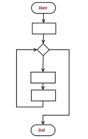
Flowchart
Flowchart is an "Graphical representation of Algorithm or diagrammatic representation of Algorithm" is called Flowchart.
Types of Algorithm Analysis
Output:
Recursion


Thank you,
By Er. Shejwal Shrikant.
30-12-2019, Monday.
Algorithm
Algorithm is "step by step procedure to solve the problem" is called as Algorithm.
All Algorithm must satisfy the following criteria -
- 1) Input
There are more quantities that are extremely supplied. - 2) Output
At least one quantity is produced. - 3) Definiteness
Each instruction of the algorithm should be clear and unambiguous. - 4) Finiteness
The process should be terminated after a finite number of steps. - 5) Effectiveness
Every instruction must be basic enough to be carried out theoretically or by using paper and pencil.
Properties of Algorithm
Simply writing the sequence of instructions as an algorithm is not sufficient to accomplish certain task. It is necessary to have following properties associated with an algorithm.
- Non Ambiguity
Each step in an algorithm should be non-ambiguous. That means each instruction should be clear and precise. The instruction in any algorithm should not denote any conflicting meaning. This property also indicates the effectiveness of algorithm. - Range of Input
The range of input should be specified. This is because normally the algorithm is input driven and if the range of input is not being specified then algorithm can go in an infinite state. - Multiplicity
The same algorithm can be represented into several different ways. That means we can write in simple English the sequence of instruction or we can write it in form of pseudo code. Similarly, for solving the same problem we can write several different algorithms. - Speed
The algorithmis written using some specified ideas. Bus such algorithm should be efficient and should produce the output with fast speed. - Finiteness
The algorithm should be finite. That means after performing required operations it should be terminate.
Expressing Algorithms
Describing algorithms requires a notation for expressing a sequence of steps to be performed. The three most common options are (1) English, (2) pseudocode, or (3) a real programming language. Pseudocode is perhaps the most mysterious of the bunch, but it is best defined as a programming language that never complains about syntax errors. All three methods can be useful in certain circumstances, since there is a natural tradeoff between greater ease of expression and precision. English is the most natural but least precise language, while C and Pascal are precise but difficult to write and understand. Pseudocode is useful because it is a happy medium.The correct choice of which notation is best depends upon which of the three methods you are most comfortable with. I prefer to describe the ideas of an algorithm in English, moving onto a more formal, programming-language-like pseudocode to clarify sufficiently tricky details of the algorithm. A common mistake among my students is to use pseudocode to take an ill-defined idea and dress it up so that it looks more formal. In the real world, you only fool yourself when you pull this kind of stunt.
The implementation complexity of an algorithm is usually why the fastest algorithm known for a problem may not be the most appropriate for a given application. An algorithm's implementation complexity is often a function of how it has been described. Fast algorithms often make use of very complicated data structures, or use other complicated algorithms as subroutines. Turning these algorithms into programs requires building implementations of every substructure. Each catalog entry in Section
Flowchart
Flowchart is an "Graphical representation of Algorithm or diagrammatic representation of Algorithm" is called Flowchart.
Benefits of Flowchart
Let us now discuss the benefits of a flowchart.
Simplify the Logic
As it provides the pictorial representation of the steps; therefore, it simplifies the logic and subsequent steps.
Makes Communication Better
Because of having easily understandable pictorial logic and steps, it is a better and simple way of representation.
Effective Analysis
Once the flow-chart is prepared, it becomes very simple to analyze the problem in an effective way.
Useful in Coding
The flow-chart also helps in coding process efficiently, as it gives directions on what to do, when to do, and where to do. It makes the work easier.
Proper Testing
Further, flowchart also helps in finding the error (if any) in program
Applicable Documentation
Last but not the least, a flowchart also helps in preparing the proper document (once the codes are written).
Flow-Chart Symbols
The following table illustrates the symbols along with their names (used in a flow-chart) −
| Name | Symbol | Name | Symbol |
|---|---|---|---|
 | Flow Line |  | Magnetic Disk |
 | Terminal |  | Communication Link |
 | Processing |  | Offline Storage |
 | Decision |  | Annotation |
 | Connector | | Flow line |
 | Document |  | Off-Page Connector |
Sample of Flow Chart
Algorithm Design Techniques
The following is a list of several popular design approaches:
1. Divide and Conquer Approach: It is a top-down approach. The algorithms which follow the divide & conquer techniques involve three steps:
- Divide the original problem into a set of subproblems.
- Solve every subproblem individually, recursively.
- Combine the solution of the subproblems (top level) into a solution of the whole original problem.
2. Greedy Technique: Greedy method is used to solve the optimization problem. An optimization problem is one in which we are given a set of input values, which are required either to be maximized or minimized (known as objective), i.e. some constraints or conditions.
- Greedy Algorithm always makes the choice (greedy criteria) looks best at the moment, to optimize a given objective.
- The greedy algorithm doesn't always guarantee the optimal solution however it generally produces a solution that is very close in value to the optimal.
3. Dynamic Programming: Dynamic Programming is a bottom-up approach we solve all possible small problems and then combine them to obtain solutions for bigger problems.
This is particularly helpful when the number of copying subproblems is exponentially large. Dynamic Programming is frequently related to Optimization Problems.
4. Branch and Bound: In Branch & Bound algorithm a given subproblem, which cannot be bounded, has to be divided into at least two new restricted subproblems. Branch and Bound algorithm are methods for global optimization in non-convex problems. Branch and Bound algorithms can be slow, however in the worst case they require effort that grows exponentially with problem size, but in some cases we are lucky, and the method coverage with much less effort.
5. Randomized Algorithms: A randomized algorithm is defined as an algorithm that is allowed to access a source of independent, unbiased random bits, and it is then allowed to use these random bits to influence its computation.
6. Backtracking Algorithm: Backtracking Algorithm tries each possibility until they find the right one. It is a depth-first search of the set of possible solution. During the search, if an alternative doesn't work, then backtrack to the choice point, the place which presented different alternatives, and tries the next alternative.
7. Randomized Algorithm: A randomized algorithm uses a random number at least once during the computation make a decision.
Example 1: In Quick Sort, using a random number to choose a pivot.
Example 2: Trying to factor a large number by choosing a random number as possible divisors.
Performance Analysis of Algorithm
In theoretical analysis of algorithms, it is common to estimate their complexity in the asymptotic sense, i.e., to estimate the complexity function for arbitrarily large input. The term "analysis of algorithms" was coined by Donald Knuth.
Algorithm analysis is an important part of computational complexity theory, which provides theoretical estimation for the required resources of an algorithm to solve a specific computational problem. Most algorithms are designed to work with inputs of arbitrary length. Analysis of algorithms is the determination of the amount of time and space resources required to execute it.
Usually, the efficiency or running time of an algorithm is stated as a function relating the input length to the number of steps, known as time complexity, or volume of memory, known as space complexity.
The Need for Analysis
In this chapter, we will discuss the need for analysis of algorithms and how to choose a better algorithm for a particular problem as one computational problem can be solved by different algorithms.
By considering an algorithm for a specific problem, we can begin to develop pattern recognition so that similar types of problems can be solved by the help of this algorithm.
Algorithms are often quite different from one another, though the objective of these algorithms are the same. For example, we know that a set of numbers can be sorted using different algorithms. Number of comparisons performed by one algorithm may vary with others for the same input. Hence, time complexity of those algorithms may differ. At the same time, we need to calculate the memory space required by each algorithm.
Analysis of algorithm is the process of analyzing the problem-solving capability of the algorithm in terms of the time and size required (the size of memory for storage while implementation). However, the main concern of analysis of algorithms is the required time or performance. Generally, we perform the following types of analysis −
- Worst-case − The maximum number of steps taken on any instance of size a.
- Best-case − The minimum number of steps taken on any instance of size a.
- Average case − An average number of steps taken on any instance of size a.
- Amortized − A sequence of operations applied to the input of size a averaged over time.
To solve a problem, we need to consider time as well as space complexity as the program may run on a system where memory is limited but adequate space is available or may be vice-versa. In this context, if we compare bubble sort and merge sort. Bubble sort does not require additional memory, but merge sort requires additional space. Though time complexity of bubble sort is higher compared to merge sort, we may need to apply bubble sort if the program needs to run in an environment, where memory is very limited.
Types of Algorithm Analysis
We can have three cases to analyze an algorithm:
1) Worst Case
2) Average Case
3) Best Case
1) Worst Case
2) Average Case
3) Best Case
Let us consider the following implementation of Linear Search.
// C implementation of the approach #include <stdio.h> // Linearly search x in arr[]. // If x is present then return the index, // otherwise return -1 int search(int arr[], int n, int x)
{ int i;
for (i=0; i<n; i++)
{
if (arr[i] == x)
return i;
}
return -1;
} /* Driver program to test above functions*/int main()
{ int arr[] = {1, 10, 30, 15};
int x = 30;
int n = sizeof(arr)/sizeof(arr[0]);
printf("%d is present at index %d", x, search(arr, n, x));
getchar();
return 0;
} |
Output:
30 is present at index 2
Worst Case Analysis (Usually Done)
In the worst case analysis, we calculate upper bound on running time of an algorithm. We must know the case that causes maximum number of operations to be executed. For Linear Search, the worst case happens when the element to be searched (x in the above code) is not present in the array. When x is not present, the search() functions compares it with all the elements of arr[] one by one. Therefore, the worst case time complexity of linear search would be Θ(n).
In the worst case analysis, we calculate upper bound on running time of an algorithm. We must know the case that causes maximum number of operations to be executed. For Linear Search, the worst case happens when the element to be searched (x in the above code) is not present in the array. When x is not present, the search() functions compares it with all the elements of arr[] one by one. Therefore, the worst case time complexity of linear search would be Θ(n).
Average Case Analysis (Sometimes done)
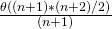
In average case analysis, we take all possible inputs and calculate computing time for all of the inputs. Sum all the calculated values and divide the sum by total number of inputs. We must know (or predict) distribution of cases. For the linear search problem, let us assume that all cases are uniformly distributed (including the case of x not being present in array). So we sum all the cases and divide the sum by (n+1). Following is the value of average case time complexity.
In average case analysis, we take all possible inputs and calculate computing time for all of the inputs. Sum all the calculated values and divide the sum by total number of inputs. We must know (or predict) distribution of cases. For the linear search problem, let us assume that all cases are uniformly distributed (including the case of x not being present in array). So we sum all the cases and divide the sum by (n+1). Following is the value of average case time complexity.
Average Case Time =

                  =

                  = Θ(n)

Best Case Analysis (Bogus)
In the best case analysis, we calculate lower bound on running time of an algorithm. We must know the case that causes minimum number of operations to be executed. In the linear search problem, the best case occurs when x is present at the first location. The number of operations in the best case is constant (not dependent on n). So time complexity in the best case would be Θ(1)
Most of the times, we do worst case analysis to analyze algorithms. In the worst analysis, we guarantee an upper bound on the running time of an algorithm which is good information.
The average case analysis is not easy to do in most of the practical cases and it is rarely done. In the average case analysis, we must know (or predict) the mathematical distribution of all possible inputs.
The Best Case analysis is bogus. Guaranteeing a lower bound on an algorithm doesn’t provide any information as in the worst case, an algorithm may take years to run.
For some algorithms, all the cases are asymptotically same, i.e., there are no worst and best cases. For example, Merge Sort. Merge Sort does Θ(nLogn) operations in all cases. Most of the other sorting algorithms have worst and best cases. For example, in the typical implementation of Quick Sort (where pivot is chosen as a corner element), the worst occurs when the input array is already sorted and the best occur when the pivot elements always divide array in two halves. For insertion sort, the worst case occurs when the array is reverse sorted and the best case occurs when the array is sorted in the same order as output.
Asymptotic Notations
are the expressions that are used to represent the complexity of an algorithm.
As we discussed in the last tutorial, there are three types of analysis that we perform on a particular algorithm.
Best Case: In which we analyse the performance of an algorithm for the input, for which the algorithm takes less time or space.
Best Case: In which we analyse the performance of an algorithm for the input, for which the algorithm takes less time or space.
Worst Case: In which we analyse the performance of an algorithm for the input, for which the algorithm takes long time or space.
Average Case: In which we analyse the performance of an algorithm for the input, for which the algorithm takes time or space that lies between best and worst case.
Types of Asymptotic Notation
1. Big-O Notation (Ο) – Big O notation specifically describes worst case scenario.
2. Omega Notation (Ω) – Omega(Ω) notation specifically describes best case scenario.
3. Theta Notation (θ) – This notation represents the average complexity of an algorithm.
2. Omega Notation (Ω) – Omega(Ω) notation specifically describes best case scenario.
3. Theta Notation (θ) – This notation represents the average complexity of an algorithm.
Big-O Notation (Ο)
Big O notation specifically describes worst case scenario. It represents the upper bound running time complexity of an algorithm. Lets take few examples to understand how we represent the time and space complexity using Big O notation.
O(1)
Big O notation O(1) represents the complexity of an algorithm that always execute in same time or space regardless of the input data.
O(1) example
The following step will always execute in same time(or space) regardless of the size of input data.
The following step will always execute in same time(or space) regardless of the size of input data.
Accessing array index(int num = arr[5])
O(n)
Big O notation O(N) represents the complexity of an algorithm, whose performance will grow linearly (in direct proportion) to the size of the input data.
O(n) example
The execution time will depend on the size of array. When the size of the array increases, the execution time will also increase in the same proportion (linearly)
The execution time will depend on the size of array. When the size of the array increases, the execution time will also increase in the same proportion (linearly)
Traversing an array
O(n^2)
Big O notation O(n^2) represents the complexity of an algorithm, whose performance is directly proportional to the square of the size of the input data.
O(n^2) example
Traversing a 2D array
Other examples: Bubble sort, insertion sort and selection sort algorithms (we will discuss these algorithms later in separate tutorials)
Similarly there are other Big O notations such as:
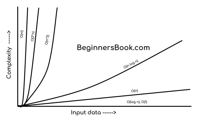
logarithmic growth O(log n), log-linear growth O(n log n), exponential growth O(2^n) and factorial growth O(n!).
logarithmic growth O(log n), log-linear growth O(n log n), exponential growth O(2^n) and factorial growth O(n!).
If I have to draw a diagram to compare the performance of algorithms denoted by these notations, then I would draw it like this:
O(1) < O(log n) < O (n) < O(n log n) < O(n^2) < O (n^3)< O(2^n) < O(n!)
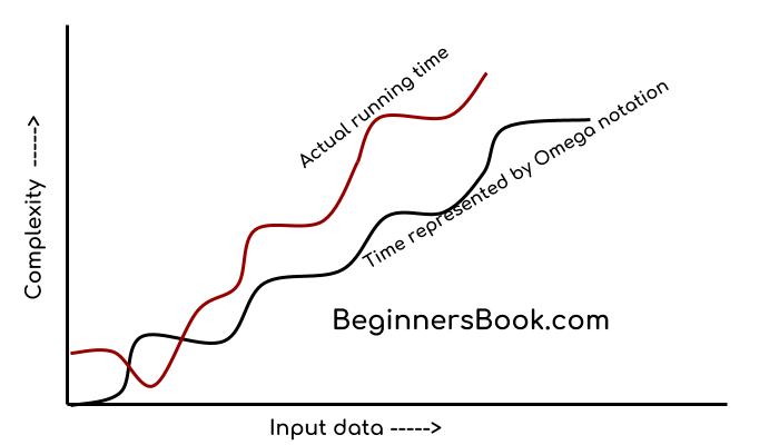
Omega Notation (Ω)
Omega notation specifically describes best case scenario. It represents the lower bound running time complexity of an algorithm. So if we represent a complexity of an algorithm in Omega notation, it means that the algorithm cannot be completed in less time than this, it would at-least take the time represented by Omega notation or it can take more (when not in best case scenario).
Theta Notation (θ)
This notation describes both upper bound and lower bound of an algorithm so we can say that it defines exact asymptotic behaviour. In the real case scenario the algorithm not always run on best and worst cases, the average running time lies between best and worst and can be represented by the theta notation.

Recursion
Some computer programming languages allow a module or function to call itself. This technique is known as recursion. In recursion, a function α either calls itself directly or calls a function β that in turn calls the original function α. The function α is called recursive function.
Example − a function calling itself.
int function(int value) {
   if(value < 1)
      return;
   function(value - 1);

   printf("%d ",value);
}
Example − a function that calls another function which in turn calls it again.
int function1(int value1) {
   if(value1 < 1)
      return;
   function2(value1 - 1);
   printf("%d ",value1);
}
int function2(int value2) {
   function1(value2);
}
Properties of Recursion
A recursive function can go infinite like a loop. To avoid infinite running of recursive function, there are two properties that a recursive function must have −
- Base criteria − There must be at least one base criteria or condition, such that, when this condition is met the function stops calling itself recursively.
- Progressive approach − The recursive calls should progress in such a way that each time a recursive call is made it comes closer to the base criteria.
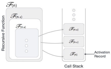
Implementation of Recursion
Many programming languages implement recursion by means of stacks. Generally, whenever a function (caller) calls another function (callee) or itself as callee, the caller function transfers execution control to the callee. This transfer process may also involve some data to be passed from the caller to the callee.
This implies, the caller function has to suspend its execution temporarily and resume later when the execution control returns from the callee function. Here, the caller function needs to start exactly from the point of execution where it puts itself on hold. It also needs the exact same data values it was working on. For this purpose, an activation record (or stack frame) is created for the caller function.
This activation record keeps the information about local variables, formal parameters, return address and all information passed to the caller function.
Analysis of Recursion
One may argue why to use recursion, as the same task can be done with iteration. The first reason is, recursion makes a program more readable and because of latest enhanced CPU systems, recursion is more efficient than iterations.
Time Complexity
In case of iterations, we take number of iterations to count the time complexity. Likewise, in case of recursion, assuming everything is constant, we try to figure out the number of times a recursive call is being made. A call made to a function is Ο(1), hence the (n) number of times a recursive call is made makes the recursive function Ο(n).
Space Complexity
Space complexity is counted as what amount of extra space is required for a module to execute. In case of iterations, the compiler hardly requires any extra space. The compiler keeps updating the values of variables used in the iterations. But in case of recursion, the system needs to store activation record each time a recursive call is made. Hence, it is considered that space complexity of recursive function may go higher than that of a function with iteration.
Recurrence Relation
A recurrence is an equation or inequality that describes a function in terms of its values on smaller inputs. To solve a Recurrence Relation means to obtain a function defined on the natural numbers that satisfy the recurrence.
For Example, the Worst Case Running Time T(n) of the MERGE SORT Procedures is described by the recurrence.
T (n) = θ (1) if n=1 2T+ θ (n) if n>1
There are four methods for solving Recurrence:
1. Substitution Method:
The Substitution Method Consists of two main steps:
- Guess the Solution.
- Use the mathematical induction to find the boundary condition and shows that the guess is correct.
For Example1 Solve the equation by Substitution Method.
T (n) = T
We have to show that it is asymptotically bound by O (log n).
Solution:
For T (n) = O (log n)
We have to show that for some constant c
- T (n) ≤c logn.
Put this in given Recurrence Equation.
T (n) ≤c log
Example2 Consider the Recurrence
T (n) = 2T
Find an Asymptotic bound on T.
Solution:
We guess the solution is O (n (logn)).Thus for constant 'c'. T (n) ≤c n logn Put this in given Recurrence Equation. Now, T (n) ≤2c
2. Iteration Methods
It means to expand the recurrence and express it as a summation of terms of n and initial condition.
Example1: Consider the Recurrence
- T (n) = 1 if n=1
- = 2T (n-1) if n>1
Solution:
T (n) = 2T (n-1)
      = 2[2T (n-2)] = 22T (n-2)
      = 4[2T (n-3)] = 23T (n-3)
      = 8[2T (n-4)] = 24T (n-4)   (Eq.1)

Repeat the procedure for i times

T (n) = 2i T (n-i)
Put n-i=1 or i= n-1 in    (Eq.1)
T (n) = 2n-1 T (1)
      = 2n-1 .1    {T (1) =1 .....given}
      = 2n-1
Example2: Consider the Recurrence
- T (n) = T (n-1) +1 and T (1) = θ (1).
Solution:
 T (n) = T (n-1) +1
       = (T (n-2) +1) +1 = (T (n-3) +1) +1+1
       = T (n-4) +4 = T (n-5) +1+4
       = T (n-5) +5= T (n-k) + k
Where k = n-1
   T (n-k) = T (1) = θ (1)
   T (n) = θ (1) + (n-1) = 1+n-1=n= θ (n).
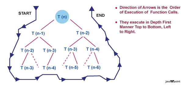
3. Recursion Tree Method
1. Recursion Tree Method is a pictorial representation of an iteration method which is in the form of a tree where at each level nodes are expanded.
2. In general, we consider the second term in recurrence as root.
3. It is useful when the divide & Conquer algorithm is used.
4. It is sometimes difficult to come up with a good guess. In Recursion tree, each root and child represents the cost of a single subproblem.
5. We sum the costs within each of the levels of the tree to obtain a set of pre-level costs and then sum all pre-level costs to determine the total cost of all levels of the recursion.
6. A Recursion Tree is best used to generate a good guess, which can be verified by the Substitution Method.
Example 1
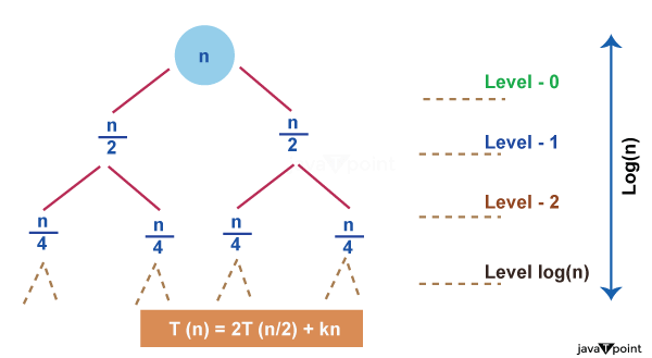
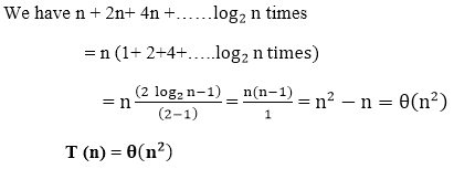
Consider T (n) = 2T
We have to obtain the asymptotic bound using recursion tree method.
Solution: The Recursion tree for the above recurrence is
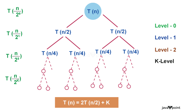
Example 2: Consider the following recurrence
T (n) = 4T
Obtain the asymptotic bound using recursion tree method.
Solution: The recursion trees for the above recurrence
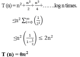
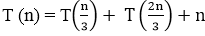
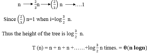
Example 3: Consider the following recurrence
Obtain the asymptotic bound using recursion tree method.
Solution: The given Recurrence has the following recursion tree
When we add the values across the levels of the recursion trees, we get a value of n for every level. The longest path from the root to leaf is
4. Master Method
The Master Method is used for solving the following types of recurrence
T (n) = a T + f (n) with a≥1 and b≥1 be constant & f(n) be a function and
  can be interpreted as
+ f (n) with a≥1 and b≥1 be constant & f(n) be a function and can be interpreted as
Let T (n) is defined on non-negative integers by the recurrence.
T (n) = a T
In the function to the analysis of a recursive algorithm, the constants and function take on the following significance:
- n is the size of the problem.
- a is the number of subproblems in the recursion.
- n/b is the size of each subproblem. (Here it is assumed that all subproblems are essentially the same size.)
- f (n) is the sum of the work done outside the recursive calls, which includes the sum of dividing the problem and the sum of combining the solutions to the subproblems.
- It is not possible always bound the function according to the requirement, so we make three cases which will tell us what kind of bound we can apply on the function.
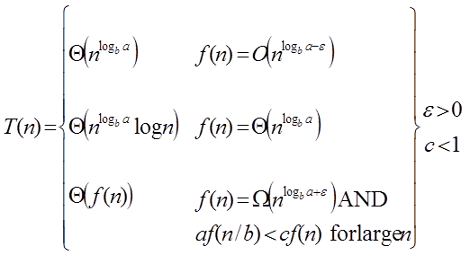
Master Theorem:
It is possible to complete an asymptotic tight bound in these three cases:
Case1: If f (n) = 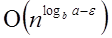 for some constant ε >0, then it follows that:
for some constant ε >0, then it follows that:T (n) = Θ
Example:
T (n) = 8 Tapply master theorem on it.
Solution:
Compare T (n) = 8 Ta = 8, b=2, f (n) = 1000 n2, logba = log28 = 3 Put all the values in: f (n) =
1000 n2 = O (n3-ε ) If we choose ε=1, we get: 1000 n2 = O (n3-1) = O (n2)
Since this equation holds, the first case of the master theorem applies to the given recurrence relation, thus resulting in the conclusion:
T (n) = ΘTherefore: T (n) = Θ (n3)
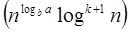
Case 2: If it is true, for some constant k ≥ 0 that:
F (n) = Θthen it follows that: T (n) = Θ
Example:
T (n) = 2, solve the recurrence by using the master method. As compare the given problem with T (n) = a T
a = 2, b=2, k=0, f (n) = 10n, logba = log22 =1 Put all the values in f (n) =Θ
, we will get 10n = Θ (n1) = Θ (n) which is true. Therefore: T (n) = Θ
= Θ (n log n)
Case 3: If it is true f(n) = Ω  for some constant ε >0 and it also true that: a f
  for some constant c<1 for large value of n ,then :
for some constant ε >0 and it also true that: a f for some constant c<1 for large value of n ,then :- T (n) = Θ((f (n))
Example: Solve the recurrence relation:
T (n) = 2
Solution:
Compare the given problem with T (n) = a Ta= 2, b =2, f (n) = n2, logba = log22 =1 Put all the values in f (n) = Ω
..... (Eq. 1) If we insert all the value in (Eq.1), we will get n2 = Ω(n1+ε) put ε =1, then the equality will hold. n2 = Ω(n1+1) = Ω(n2) Now we will also check the second condition: 2
If we will choose c =1/2, it is true:
∀ n ≥1 So it follows: T (n) = Θ ((f (n)) T (n) = Θ(n2)
Heap Sort
Binary Heap:
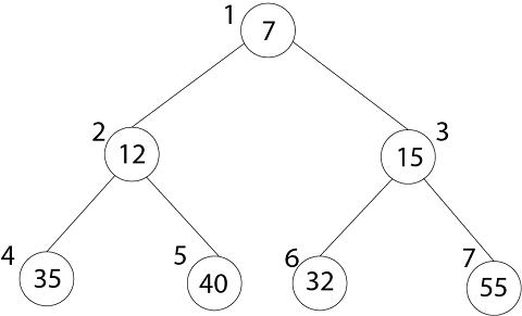
Binary Heap is an array object can be viewed as Complete Binary Tree. Each node of the Binary Tree corresponds to an element in an array.
- Length [A],number of elements in array
- Heap-Size[A], number of elements in a heap stored within array A.
The root of tree A [1] and gives index 'i' of a node that indices of its parents, left child, and the right child can be computed.
- PARENT (i)
- Return floor (i/2)
- LEFT (i)
- Return 2i
- RIGHT (i)
- Return 2i+1
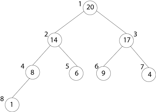
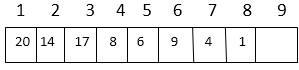
Representation of an array of the above figure is given below:
The index of 20 is 1
To find the index of the left child, we calculate 1*2=2
This takes us (correctly) to the 14.
Now, we go right, so we calculate 2*2+1=5
This takes us (again, correctly) to the 6.
Now, 4's index is 7, we want to go to the parent, so we calculate 7/2 =3 which takes us to the 17.
Heap Property:
A binary heap can be classified as Max Heap or Min Heap
1. Max Heap: In a Binary Heap, for every node I other than the root, the value of the node is greater than or equal to the value of its highest child
- A [PARENT (i) ≥A[i]
Thus, the highest element in a heap is stored at the root. Following is an example of MAX-HEAP
2. MIN-HEAP: In MIN-HEAP, the value of the node is lesser than or equal to the value of its lowest child.
- A [PARENT (i) ≤A[i]
Heapify Method:
1. Maintaining the Heap Property: Heapify is a procedure for manipulating heap Data Structure. It is given an array A and index I into the array. The subtree rooted at the children of A [i] are heap but node A [i] itself may probably violate the heap property i.e. A [i] < A [2i] or A [2i+1]. The procedure 'Heapify' manipulates the tree rooted as A [i] so it becomes a heap.
MAX-HEAPIFY (A, i)
 1. l ← left [i]
 2. r ← right [i]
 3. if l≤ heap-size [A] and A[l] > A [i]
 4. then largest ← l
 5. Else largest ← i
 6. If r≤ heap-size [A] and A [r] > A[largest]
 7. Then largest ← r
 8. If largest ≠ i
 9. Then exchange A [i]    A [largest]
 10. MAX-HEAPIFY (A, largest)
Analysis:
The maximum levels an element could move up are Θ (log n) levels. At each level, we do simple comparison which O (1). The total time for heapify is thus O (log n).
Building a Heap:
BUILDHEAP (array A, int n)
 1 for i ← n/2 down to 1
 2 do
 3 HEAPIFY (A, i, n)
HEAP-SORT ALGORITHM:
HEAP-SORT (A)
 1. BUILD-MAX-HEAP (A)
 2. For I ← length[A] down to Z
 3. Do exchange A [1] ←→ A [i]
 4. Heap-size [A] ← heap-size [A]-1
 5. MAX-HEAPIFY (A,1)
Analysis: Build max-heap takes O (n) running time. The Heap Sort algorithm makes a call to 'Build Max-Heap' which we take O (n) time & each of the (n-1) calls to Max-heap to fix up a new heap. We know 'Max-Heapify' takes time O (log n)
The total running time of Heap-Sort is O (n log n).
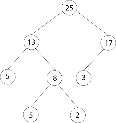
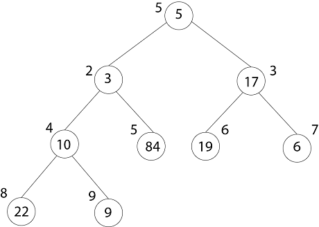
Example: Illustrate the Operation of BUILD-MAX-HEAP on the array.
- A = (5, 3, 17, 10, 84, 19, 6, 22, 9)
Solution: Originally:
- Heap-Size (A) =9, so first we call MAX-HEAPIFY (A, 4)
- And I = 4.5= 4 to 1
- After MAX-HEAPIFY (A, 4) and i=4
- L ← 8, r ← 9
- l≤ heap-size[A] and A [l] >A [i]
- 8 ≤9 and 22>10
- Then Largest ← 8
- If r≤ heap-size [A] and A [r] > A [largest]
- 9≤9 and 9>22
- If largest (8) ≠4
- Then exchange A [4] ←→ A [8]
- MAX-HEAPIFY (A, 8)
- After MAX-HEAPIFY (A, 3) and i=3
- l← 6, r ← 7
- l≤ heap-size[A] and A [l] >A [i]
- 6≤ 9 and 19>17
- Largest ← 6
- If r≤ heap-size [A] and A [r] > A [largest]
- 7≤9 and 6>19
- If largest (6) ≠3
- Then Exchange A [3] ←→ A [6]
- MAX-HEAPIFY (A, 6)
- After MAX-HEAPIFY (A, 2) and i=2
- l ← 4, r ← 5
- l≤ heap-size[A] and A [l] >A [i]
- 4≤9 and 22>3
- Largest ← 4
- If r≤ heap-size [A] and A [r] > A [largest]
- 5≤9 and 84>22
- Largest ← 5
- If largest (4) ≠2
- Then Exchange A [2] ←→ A [5]
- MAX-HEAPIFY (A, 5)
- After MAX-HEAPIFY (A, 1) and i=1
- l ← 2, r ← 3
- l≤ heap-size[A] and A [l] >A [i]
- 2≤9 and 84>5
- Largest ← 2
- If r≤ heap-size [A] and A [r] > A [largest]
- 3≤9 and 19<84
- If largest (2) ≠1
- Then Exchange A [1] ←→ A [2]
- MAX-HEAPIFY (A, 2)
Thank you,
By Er. Shejwal Shrikant.
30-12-2019, Monday.

Comments
Post a Comment