Dynamic Programming

                            Dynamic Programming

Introduction of Dynamic Programming

Dynamic Programming is the most powerful design technique for solving optimization problems.

Divide & Conquer algorithm partition the problem into disjoint subproblems solve the subproblems recursively and then combine their solution to solve the original problems.

Dynamic Programming is used when the subproblems are not independent, e.g. when they share the same subproblems. In this case, divide and conquer may do more work than necessary, because it solves the same sub problem multiple times.

Dynamic Programming solves each subproblems just once and stores the result in a table so that it can be repeatedly retrieved if needed again.

Dynamic Programming is a Bottom-up approach- we solve all possible small problems and then combine to obtain solutions for bigger problems.

Dynamic Programming is a paradigm of algorithm design in which an optimization problem is solved by a combination of achieving sub-problem solutions and appearing to the "principle of optimality".

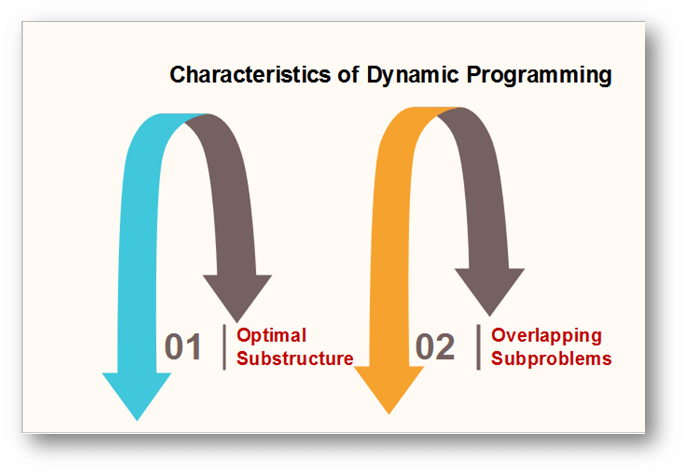
Characteristics of Dynamic Programming:

Dynamic Programming works when a problem has the following features:-

• Optimal Substructure: If an optimal solution contains optimal sub solutions then a problem exhibits optimal substructure.
• Overlapping subproblems: When a recursive algorithm would visit the same subproblems repeatedly, then a problem has overlapping subproblems.

If a problem has optimal substructure, then we can recursively define an optimal solution. If a problem has overlapping subproblems, then we can improve on a recursive implementation by computing each subproblem only once.

If a problem doesn't have optimal substructure, there is no basis for defining a recursive algorithm to find the optimal solutions. If a problem doesn't have overlapping sub problems, we don't have anything to gain by using dynamic programming.

If the space of subproblems is enough (i.e. polynomial in the size of the input), dynamic programming can be much more efficient than recursion.

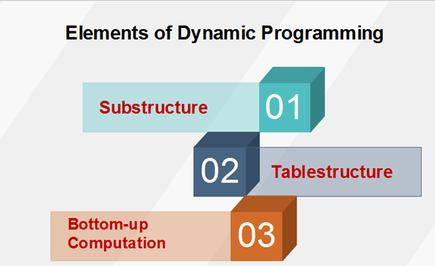
Elements of Dynamic Programming

There are basically three elements that characterize a dynamic programming algorithm:-

1. Substructure: Decompose the given problem into smaller subproblems. Express the solution of the original problem in terms of the solution for smaller problems.
2. Table Structure: After solving the sub-problems, store the results to the sub problems in a table. This is done because subproblem solutions are reused many times, and we do not want to repeatedly solve the same problem over and over again.
3. Bottom-up Computation: Using table, combine the solution of smaller subproblems to solve larger subproblems and eventually arrives at a solution to complete problem.

Note: Bottom-up means:-

1. Start with smallest subproblems.
2. Combining their solutions obtain the solution to sub-problems of increasing size.
3. Until solving at the solution of the original problem.

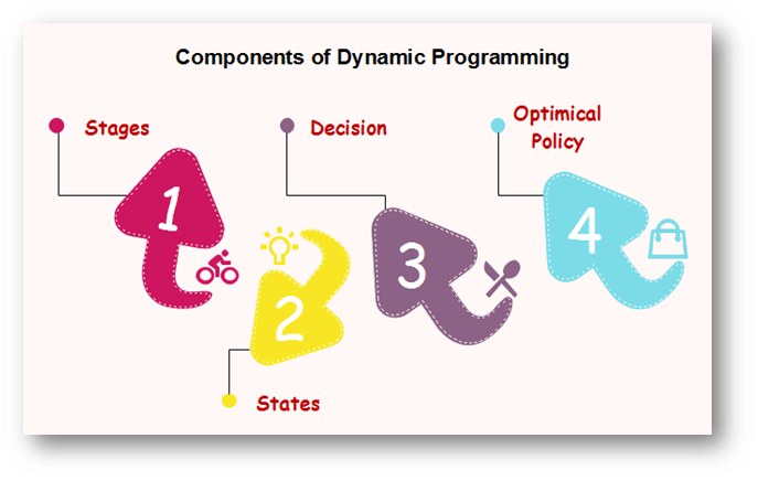
Components of Dynamic programming

1. Stages: The problem can be divided into several subproblems, which are called stages. A stage is a small portion of a given problem. For example, in the shortest path problem, they were defined by the structure of the graph.
2. States: Each stage has several states associated with it. The states for the shortest path problem was the node reached.
3. Decision: At each stage, there can be multiple choices out of which one of the best decisions should be taken. The decision taken at every stage should be optimal; this is called a stage decision.
4. Optimal policy: It is a rule which determines the decision at each stage; a policy is called an optimal policy if it is globally optimal. This is known as Bellman principle of optimality.
5. Given the current state, the optimal choices for each of the remaining states does not depend on the previous states or decisions. In the shortest path problem, it was not necessary to know how we got a node only that we did.
6. There exist a recursive relationship that identify the optimal decisions for stage j, given that stage j+1, has already been solved.
7. The final stage must be solved by itself.

Development of Dynamic Programming Algorithm

It can be broken into four steps:

1. Characterize the structure of an optimal solution.
2. Recursively defined the value of the optimal solution. Like Divide and Conquer, divide the problem into two or more optimal parts recursively. This helps to determine what the solution will look like.
3. Compute the value of the optimal solution from the bottom up (starting with the smallest subproblems)
4. Construct the optimal solution for the entire problem form the computed values of smaller subproblems.

Applications of dynamic programming

1. 0/1 knapsack problem
2. Mathematical optimization problem
3. All pair Shortest path problem
4. Reliability design problem
5. Longest common subsequence (LCS)
6. Flight control and robotics control
7. Time-sharing: It schedules the job to maximize CPU usage

Differentiate between Divide & Conquer Method vs Dynamic Programming.

Divide & Conquer Method	Dynamic Programming
1.It deals (involves) three steps at each level of recursion: Divide the problem into a number of subproblems. Conquer the subproblems by solving them recursively. Combine the solution to the subproblems into the solution for original subproblems.	1.It involves the sequence of four steps: Characterize the structure of optimal solutions. Recursively defines the values of optimal solutions. Compute the value of optimal solutions in a Bottom-up minimum. Construct an Optimal Solution from computed information.
2. It is Recursive.	2. It is non Recursive.
3. It does more work on subproblems and hence has more time consumption.	3. It solves subproblems only once and then stores in the table.
4. It is a top-down approach.	4. It is a Bottom-up approach.
5. In this subproblems are independent of each other.	5. In this subproblems are interdependent.
6. For example: Merge Sort & Binary Search etc.	6. For example: Matrix Multiplication.

Matrix Chain Multiplication

It is a Method under Dynamic Programming in which previous output is taken as input for next.

Here, Chain means one matrix's column is equal to the second matrix's row [always].

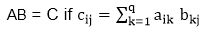
In general:

If A = ⌊aij⌋ is a p x q matrix 
   B = ⌊bij⌋ is a q x r matrix
   C = ⌊cij⌋ is a p x r matrix

Then

Given following matrices {A₁,A₂,A₃,...A_n} and we have to perform the matrix multiplication, which can be accomplished by a series of matrix multiplications

A1 xA2 x,A3 x.....x An

Matrix Multiplication operation is associative in nature rather commutative. By this, we mean that we have to follow the above matrix order for multiplication but we are free to parenthesize the above multiplication depending upon our need.

In general, for 1≤ i≤ p and 1≤ j ≤ r

It can be observed that the total entries in matrix 'C' is 'pr' as the matrix is of dimension p x r Also each entry takes O (q) times to compute, thus the total time to compute all possible entries for the matrix 'C' which is a multiplication of 'A' and 'B' is proportional to the product of the dimension p q r.

It is also noticed that we can save the number of operations by reordering the parenthesis.

Example1: Let us have 3 matrices, A₁,A₂,A₃ of order (10 x 100), (100 x 5) and (5 x 50) respectively.

Three Matrices can be multiplied in two ways:

1. A₁,(A₂,A₃): First multiplying(A₂ and A₃) then multiplying and resultant withA₁.
2. (A₁,A₂),A₃: First multiplying(A₁ and A₂) then multiplying and resultant withA₃.

No of Scalar multiplication in Case 1 will be:

1. (100 x 5 x 50) + (10 x 100 x 50) = 25000 + 50000 = 75000  

No of Scalar multiplication in Case 2 will be:

1. (100 x 10 x 5) + (10 x 5 x 50) = 5000 + 2500 = 7500  

To find the best possible way to calculate the product, we could simply parenthesis the expression in every possible fashion and count each time how many scalar multiplication are required.

Matrix Chain Multiplication Problem can be stated as "find the optimal parenthesization of a chain of matrices to be multiplied such that the number of scalar multiplication is minimized".

Number of ways for parenthesizing the matrices:

There are very large numbers of ways of parenthesizing these matrices. If there are n items, there are (n-1) ways in which the outer most pair of parenthesis can place.

(A1) (A2,A3,A4,................An)
Or (A1,A2)  (A3,A4 .................An)
Or (A1,A2,A3)  (A4 ...............An)
........................

Or(A1,A2,A3.............An-1) (An)

It can be observed that after splitting the kth matrices, we are left with two parenthesized sequence of matrices: one consist 'k' matrices and another consist 'n-k' matrices.

Now there are 'L' ways of parenthesizing the left sublist and 'R' ways of parenthesizing the right sublist then the Total will be L.R:

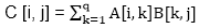
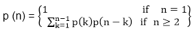
Also p (n) = c (n-1) where c (n) is the nth Catalon number

c (n) = 

On applying Stirling's formula we have

c (n) = Ω 

Which shows that 4ⁿ grows faster, as it is an exponential function, then n^1.5.

---

Development of Dynamic Programming Algorithm

1. Characterize the structure of an optimal solution.
2. Define the value of an optimal solution recursively.
3. Compute the value of an optimal solution in a bottom-up fashion.
4. Construct the optimal solution from the computed information.

---

Dynamic Programming Approach

Let A_i,j be the result of multiplying matrices i through j. It can be seen that the dimension of A_i,j is p_i-1 x p_j matrix.

Dynamic Programming solution involves breaking up the problems into subproblems whose solution can be combined to solve the global problem.

At the greatest level of parenthesization, we multiply two matrices

A1.....n=A1....k x Ak+1....n)

Thus we are left with two questions:

• How to split the sequence of matrices?
• How to parenthesize the subsequence A_1.....k andA_k+1......n?

One possible answer to the first question for finding the best value of 'k' is to check all possible choices of 'k' and consider the best among them. But that it can be observed that checking all possibilities will lead to an exponential number of total possibilities. It can also be noticed that there exists only O (n² ) different sequence of matrices, in this way do not reach the exponential growth.

Step1: Structure of an optimal parenthesization: Our first step in the dynamic paradigm is to find the optimal substructure and then use it to construct an optimal solution to the problem from an optimal solution to subproblems.

Let A_i....j where i≤ j denotes the matrix that results from evaluating the product

A_i A_i+1....A_j.

If i < j then any parenthesization of the product A_i A_i+1 ......A_j must split that the product between A_k and A_k+1 for some integer k in the range i ≤ k ≤ j. That is for some value of k, we first compute the matrices A_i.....k & A_k+1....j and then multiply them together to produce the final product A_i....j. The cost of computing A_i....k plus the cost of computing A_k+1....j plus the cost of multiplying them together is the cost of parenthesization.

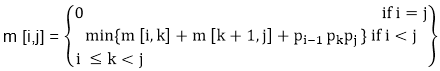
Step 2: A Recursive Solution: Let m [i, j] be the minimum number of scalar multiplication needed to compute the matrixA_i....j.

If i=j the chain consist of just one matrix A_i....i=A_i so no scalar multiplication are necessary to compute the product. Thus m [i, j] = 0 for i= 1, 2, 3....n.

If i<j we assume that to optimally parenthesize the product we split it between A_k and A_k+1 where i≤ k ≤j. Then m [i,j] equals the minimum cost for computing the subproducts A_i....k and A_k+1....j+ cost of multiplying them together. We know A_i has dimension p_i-1 x p_i, so computing the product A_i....k and A_k+1....jtakes p_i-1 p_k p_j scalar multiplication, we obtain

m [i,j] = m [i, k] + m [k + 1, j] + pi-1  pk pj

There are only (j-1) possible values for 'k' namely k = i, i+1.....j-1. Since the optimal parenthesization must use one of these values for 'k' we need only check them all to find the best.

So the minimum cost of parenthesizing the product A_i A_i+1......A_j becomes

To construct an optimal solution, let us define s [i,j] to be the value of 'k' at which we can split the product A_i A_i+1 .....A_j To obtain an optimal parenthesization i.e. s [i, j] = k such that

m[i, j] = m[i, k]+m[k+1, j]+Pi-1 Pk Pj

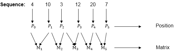
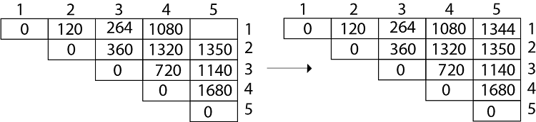
Example of Matrix Chain Multiplication

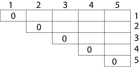
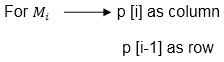
Example: We are given the sequence {4, 10, 3, 12, 20, and 7}. The matrices have size 4 x 10, 10 x 3, 3 x 12, 12 x 20, 20 x 7. We need to compute M [i,j], 0 ≤ i, j≤ 5. We know M [i, i] = 0 for all i.

Let us proceed with working away from the diagonal. We compute the optimal solution for the product of 2 matrices.

Here P₀ to P₅ are Position and M₁ to M₅ are matrix of size (p_i to p_i-1)
On the basis of sequence, we make a formula

In Dynamic Programming, initialization of every method done by '0'.So we initialize it by '0'.It will sort out diagonally.
We have to sort out all the combination but the minimum output combination is taken into consideration.

Calculation of Product of 2 matrices:
1. m (1,2) = m1  x m2
           = 4 x 10 x  10 x 3
           = 4 x 10 x 3 = 120
     
2. m (2, 3) = m2 x m3
            = 10 x 3  x  3 x 12
            = 10 x 3 x 12 = 360
   
3. m (3, 4) = m3 x m4 
            = 3 x 12  x  12 x 20
            = 3 x 12 x 20 = 720
   
4. m (4,5) = m4 x m5
           = 12 x 20  x  20 x 7
           = 12 x 20 x 7 = 1680

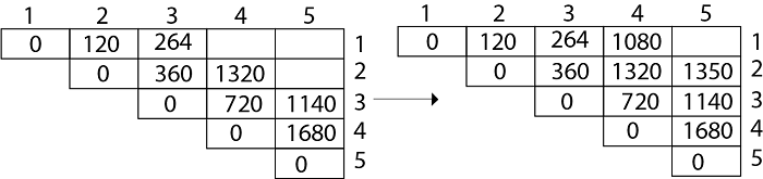
• We initialize the diagonal element with equal i,j value with '0'.
• After that second diagonal is sorted out and we get all the values corresponded to it

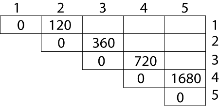
Now the third diagonal will be solved out in the same way.
Now product of 3 matrices:

M [1, 3] = M1 M2 M3

1. There are two cases by which we can solve this multiplication: ( M₁ x M₂) + M₃, M₁+ (M₂x M₃)
2. After solving both cases we choose the case in which minimum output is there.

M [1, 3] =264

As Comparing both output 264 is minimum in both cases so we insert 264 in table and ( M₁ x M₂) + M₃ this combination is chosen for the output making.

M [2, 4] = M2 M3 M4

1. There are two cases by which we can solve this multiplication: (M₂x M₃)+M₄, M₂+(M₃ x M₄)
2. After solving both cases we choose the case in which minimum output is there.

M [2, 4] = 1320

As Comparing both output 1320 is minimum in both cases so we insert 1320 in table and M₂+(M₃ x M₄) this combination is chosen for the output making.

M [3, 5] = M3  M4  M5

1. There are two cases by which we can solve this multiplication: ( M₃ x M₄) + M₅, M₃+ ( M₄xM₅)
2. After solving both cases we choose the case in which minimum output is there.

M [3, 5] = 1140

As Comparing both output 1140 is minimum in both cases so we insert 1140 in table and ( M₃ x M₄) + M₅this combination is chosen for the output making.

Now Product of 4 matrices:

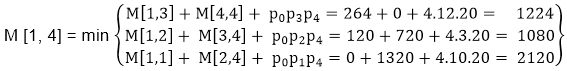
M [1, 4] = M1  M2 M3 M4

There are three cases by which we can solve this multiplication:

1. ( M₁ x M₂ x M₃) M₄
2. M₁ x(M₂ x M₃ x M₄)
3. (M₁ xM₂) x ( M₃ x M₄)

After solving these cases we choose the case in which minimum output is there

M [1, 4] =1080
As comparing the output of different cases then '1080' is minimum output, so we insert 1080 in the table and (M₁ xM₂) x (M₃ x M₄) combination is taken out in output making,

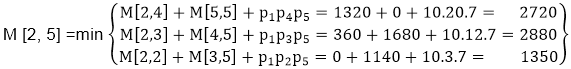
M [2, 5] = M2 M3 M4 M5

There are three cases by which we can solve this multiplication:

1. (M₂ x M₃ x M₄)x M₅
2. M₂ x( M₃ x M₄ x M₅)
3. (M₂ x M₃)x ( M₄ x M₅)

After solving these cases we choose the case in which minimum output is there

M [2, 5] = 1350

As comparing the output of different cases then '1350' is minimum output, so we insert 1350 in the table and M₂ x( M₃ x M₄ xM₅)combination is taken out in output making.

Now Product of 5 matrices:

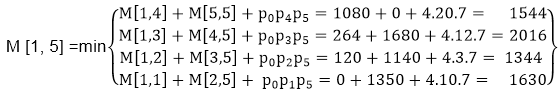
M [1, 5] = M1  M2 M3 M4 M5

There are five cases by which we can solve this multiplication:

1. (M₁ x M₂ xM₃ x M₄ )x M₅
2. M₁ x( M₂ xM₃ x M₄ xM₅)
3. (M₁ x M₂ xM₃)x M₄ xM₅
4. M₁ x M₂x(M₃ x M₄ xM₅)

After solving these cases we choose the case in which minimum output is there

M [1, 5] = 1344

As comparing the output of different cases then '1344' is minimum output, so we insert 1344 in the table and M₁ x M₂ x(M₃ x M₄ x M₅)combination is taken out in output making.
Final Output is:

Step 3: Computing Optimal Costs: let us assume that matrix A_i has dimension p_i-1x p_i for i=1, 2, 3....n. The input is a sequence (p₀,p₁,......p_n) where length [p] = n+1. The procedure uses an auxiliary table m [1....n, 1.....n] for storing m [i, j] costs an auxiliary table s [1.....n, 1.....n] that record which index of k achieved the optimal costs in computing m [i, j].

Algorithm of Matrix Chain Multiplication

MATRIX-CHAIN-ORDER (p)


 1. n   length[p]-1
 2. for i ← 1 to n
 3. do m [i, i] ← 0
 4. for l ← 2 to n    // l is the chain length
 5. do for i ← 1 to n-l + 1
 6. do j ← i+ l -1
 7. m[i,j] ←  ∞
 8. for k  ← i to j-1
 9. do q  ← m [i, k] + m [k + 1, j] + pi-1 pk pj 
 10. If q < m [i,j]
 11. then m [i,j] ← q
 12. s [i,j] ← k
 13. return m and s.      

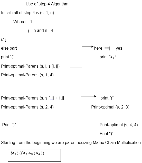
We will use table s to construct an optimal solution.
Step 1: Constructing an Optimal Solution:

PRINT-OPTIMAL-PARENS (s, i, j)
 1. if i=j
 2. then print "A"
 3. else print "("
 4. PRINT-OPTIMAL-PARENS (s, i, s [i, j])
 5. PRINT-OPTIMAL-PARENS (s, s [i, j] + 1, j)
 6. print ")"

Analysis: There are three nested loops. Each loop executes a maximum n times.

1. l, length, O (n) iterations.
2. i, start, O (n) iterations.
3. k, split point, O (n) iterations

Body of loop constant complexity
Total Complexity is: O (n³)

Algorithm with Explained Example

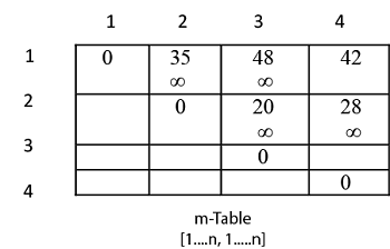
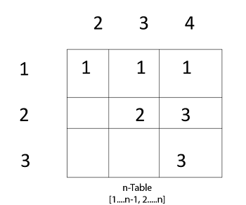
Question: P [7, 1, 5, 4, 2}
Solution: Here, P is the array of a dimension of matrices.
So here we will have 4 matrices:

A17x1  A21x5  A35x4  A44x2
i.e.
First Matrix A1 have dimension 7 x 1
Second Matrix A2 have dimension 1 x 5
Third Matrix A3 have dimension 5 x 4
Fourth Matrix A4 have dimension 4 x 2

Let say,
From P = {7, 1, 5, 4, 2} - (Given)
And P is the Position
p0 = 7, p1 =1, p2 = 5, p3 = 4, p4=2.
Length of array P = number of elements in P
∴length (p)= 5
From step 3
Follow the steps in Algorithm in Sequence
According to Step 1 of Algorithm Matrix-Chain-Order

Step 1:

 n ← length [p]-1
    Where n is the total number of elements
     And length [p] = 5
∴ n = 5 - 1 = 4
n = 4 
Now we construct two tables m and s.
Table m has dimension [1.....n, 1.......n]
Table s has dimension [1.....n-1, 2.......n] 

Now, according to step 2 of Algorithm

1. for i ← 1 to n  
2. this means: for i ← 1 to 4 (because n =4)  
3. for  i=1  
4. m [i, i]=0  
5. m [1, 1]=0  
6. Similarly for i = 2, 3, 4  
7. m [2, 2] = m [3,3] = m [4,4] = 0  
8. i.e. fill all the diagonal entries "0" in the table m  
9. Now,  
10. l ← 2 to n  
11. l ← 2 to 4    (because n =4 )  

Case 1:
1. When l - 2

    for (i ← 1 to n - l + 1)
     i ← 1 to 4 - 2 + 1
     i ← 1 to 3

When i = 1
  do   j ← i + l - 1
          j ← 1 + 2 - 1
          j ← 2
     i.e. j = 2
Now, m [i, j] ← ∞  
 i.e. m [1,2] ← ∞ 
Put ∞ in m [1, 2] table
   for k ← i to j-1
        k ← 1 to 2 - 1
        k ← 1 to 1
            k = 1
Now q ← m [i, k] + m [k + 1, j] + pi-1 pk pj
   for l = 2
        i = 1
        j =2
       k = 1
     q ← m [1,1] + m [2,2] + p0x p1x p2
             and m [1,1] = 0
    for i ← 1 to 4
     ∴ q ← 0 + 0 + 7 x 1 x 5
     q ← 35
We have m [i, j] = m [1, 2] = ∞ 
Comparing q with m [1, 2]
  q < m [i, j]
  i.e. 35 < m [1, 2]
  35 < ∞
  True
 then, m [1, 2 ] ← 35  (∴ m [i,j] ← q)
  s [1, 2] ← k
 and the value of k = 1
  s [1,2 ] ← 1
Insert "1" at dimension s [1, 2] in table s. And 35 at m [1, 2]

2. l remains 2

    L = 2
      i ← 1 to n - l + 1
      i ← 1 to 4 - 2 + 1
      i ← 1 to 3
  for i = 1 done before
  Now value of i becomes 2
  i = 2
j ←  i + l - 1
   j ←  2 + 2 - 1
   j ←  3
  j = 3
m [i , j]  ← ∞
i.e. m [2,3] ← ∞
 Initially insert ∞ at m [2, 3]
Now, for k ← i to j - 1
  k ← 2 to 3 - 1
  k ← 2 to 2
  i.e. k =2
  Now, q ← m [i, k] + m [k + 1, j] + pi-1 pk pj
  For l =2
        i = 2
        j = 3
        k = 2
  q ← m [2, 2] + m [3, 3] + p1x p2 x p3
                q ← 0 + 0 + 1 x 5 x 4
       q ← 20
       Compare q with m [i ,j ]
  If q < m [i,j]
 i.e. 20 < m [2, 3]
20 < ∞        
True
Then m [i,j ] ← q
      m [2, 3 ] ← 20
and s [2, 3] ← k
 and k = 2
s [2,3] ← 2

3. Now i become 3

  i = 3
  l = 2
j ← i + l - 1
j ← 3 + 2 - 1
j ← 4
j = 4
Now, m [i, j ] ← ∞
          m [3,4 ] ← ∞
Insert ∞ at m [3, 4] 
  for k ← i to j - 1
        k ← 3 to 4 - 1
        k ← 3 to 3
 i.e. k = 3
Now, q ← m [i, k] + m [k + 1, j] + pi-1 pk pj
i = 3
    l = 2
    j = 4
    k = 3
q ← m [3, 3] + m [4,4] + p2  x p3 x p4
q ← 0 + 0 + 5 x 2 x 4
q   40
Compare q with m [i, j]
  If q < m [i, j]
     40 < m [3, 4]
     40 < ∞ 
  True
Then, m [i,j] ← q
       m [3,4] ← 40
and s [3,4] ← k
   s [3,4] ← 3

Case 2: l becomes 3

      L = 3
       for i = 1 to n - l + 1
            i = 1 to 4 - 3 + 1
   i = 1 to 2
When i = 1
 j ← i + l - 1
 j ← 1 + 3 - 1
         j ← 3
 j = 3
Now, m [i,j]   ← ∞
          m [1, 3]  ←  ∞
for k ← i to j - 1
     k ← 1 to 3 - 1
     k ← 1 to 2

Now we compare the value for both k=1 and k = 2. The minimum of two will be placed in m [i,j] or s [i,j] respectively.

Now from above

Value of q become minimum for k=1    
  ∴ m [i,j] ← q
      m [1,3] ← 48
Also m [i,j] > q
i.e. 48 < ∞
∴ m [i , j] ← q
   m [i, j] ← 48
and s [i,j] ← k
i.e. m [1,3] ← 48
   s [1, 3] ←  1
Now i become 2
 i = 2
  l = 3
then j ← i + l -1
    j ←  2 + 3 - 1
    j ← 4
    j = 4 
    so m [i,j] ← ∞
m [2,4] ← ∞
Insert initially ∞ at m [2, 4]
      for k   ← i to j-1
       k  ← 2 to 4 - 1
       k  ← 2 to 3

Here, also find the minimum value of m [i,j] for two values of k = 2 and k =3

1. But 28 <     ∞  
2.  So m [i,j] ← q  
3.     And q  ← 28  
4. m [2, 4]  ← 28  
5. and   s [2, 4]  ← 3  
6. e. It means in s table at s [2,4] insert 3 and at m [2,4] insert 28.  

Case 3: l becomes 4

L = 4
    For i ← 1 to n-l + 1
  i ← 1 to 4 - 4 + 1
  i ← 1
  i = 1
 do j  ← i + l - 1
      j ← 1 + 4 - 1
      j ← 4
     j = 4
Now m [i,j]  ←  ∞
        m [1,4] ←  ∞
for k  ← i to j -1
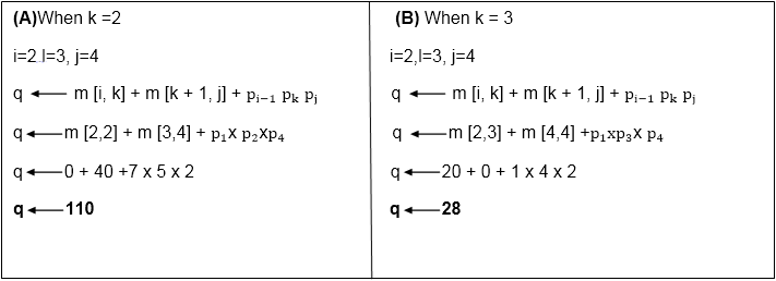
     k ← 1 to 4 - 1
     k  ← 1 to 3
When k = 1
q  ←  m [i, k] + m [k + 1, j] + pi-1 pk pj                
q  ← m [1,1] + m [2,4] + p0xp4x p1
q ← 0 + 28 + 7 x 2 x 1
q  ← 42
Compare q and m [i, j]
m [i,j] was ∞
i.e. m [1,4] 
if q < m [1,4]
   42< ∞
    True 
Then m [i,j] ← q
 m [1,4] ← 42
and s [1,4]  1 ? k =1
When k = 2
 L = 4, i=1, j = 4
q ← m [i, k] + m [k + 1, j] + pi-1 pk pj                
q ← m [1, 2] + m [3,4] + p0 xp2 xp4
q ← 35 + 40 + 7 x 5 x 2
q  ← 145
Compare q and m [i,j]
Now m [i, j]
      i.e. m [1,4] contains 42.
So if q < m [1, 4]
But 145 less than or not equal to m [1, 4]
   So 145 less than or not equal to 42.
So no change occurs.
When k = 3
 l = 4
 i = 1
 j = 4
q  ←  m [i, k] + m [k + 1, j] + pi-1 pk pj                
q ← m [1, 3] + m [4,4] + p0 xp3 x p4
q ← 48 + 0 + 7 x 4 x 2
q  ← 114
Again q less than or not equal to m [i, j]
 i.e. 114 less than or not equal to m [1, 4]
        114 less than or not equal to 42

So no change occurs. So the value of m [1, 4] remains 42. And value of s [1, 4] = 1
Now we will make use of only s table to get an optimal solution.

The algorithm first computes m [i, j] ← 0 for i=1, 2, 3.....n, the minimum costs for the chain of length 1.

Longest Common Sequence (LCS)

A subsequence of a given sequence is just the given sequence with some elements left out.
Given two sequences X and Y, we say that the sequence Z is a common sequence of X and Y if Z is a subsequence of both X and Y.
In the longest common subsequence problem, we are given two sequences X = (x₁ x₂....x_m) and Y = (y₁ y₂ y_n) and wish to find a maximum length common subsequence of X and Y. LCS Problem can be solved using dynamic programming.

---

Characteristics of Longest Common Sequence

A brute-force approach we find all the subsequences of X and check each subsequence to see if it is also a subsequence of Y, this approach requires exponential time making it impractical for the long sequence.
Given a sequence X = (x₁ x₂.....x_m) we define the ith prefix of X for i=0, 1, and 2...m as X_i= (x₁ x₂.....x_i). For example: if X = (A, B, C, B, C, A, B, C) then X₄= (A, B, C, B)

Optimal Substructure of an LCS: Let X = (x₁ x₂....x_m) and Y = (y₁ y₂.....) y_n) be the sequences and let Z = (z₁ z₂......z_k) be any LCS of X and Y.

• If x_m = y_n, then z_k=x_m=y_n and Z_k-1 is an LCS of X_m-1and Y_n-1
• If x_m ≠ y_n, then z_k≠ x_m implies that Z is an LCS of X_m-1and Y.
• If x_m ≠ y_n, then z_k≠y_n implies that Z is an LCS of X and Y_n-1

Step 2: Recursive Solution: LCS has overlapping subproblems property because to find LCS of X and Y, we may need to find the LCS of X_m-1 and Y_n-1. If x_m ≠ y_n, then we must solve two subproblems finding an LCS of X and Y_n-1.Whenever of these LCS's longer is an LCS of x and y. But each of these subproblems has the subproblems of finding the LCS of X_m-1 and Y_n-1.

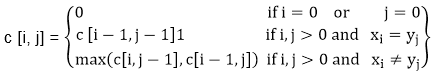
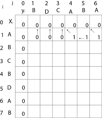
Let c [i,j] be the length of LCS of the sequence X_iand Y_j.If either i=0 and j =0, one of the sequences has length 0, so the LCS has length 0. The optimal substructure of the LCS problem given the recurrence formula

Step3: Computing the length of an LCS: let two sequences X = (x₁ x₂.....x_m) and Y = (y₁ y₂..... y_n) as inputs. It stores the c [i,j] values in the table c [0......m,0..........n].Table b [1..........m, 1..........n] is maintained which help us to construct an optimal solution. c [m, n] contains the length of an LCS of X,Y.

Algorithm of Longest Common Sequence

LCS-LENGTH (X, Y)
 1. m ← length [X]          
 2. n ← length [Y]
 3. for i ← 1 to m
 4. do c [i,0] ← 0
 5. for j ← 0 to m
 6. do c [0,j] ← 0
 7. for i ← 1 to m
 8. do for j ← 1 to n
 9. do if xi= yj 
 10. then c [i,j] ← c [i-1,j-1] + 1 
 11. b [i,j] ← "↖"
 12. else if c[i-1,j] ≥ c[i,j-1]
 13. then c [i,j] ← c [i-1,j]
 14. b [i,j] ← "↑"
 15. else c [i,j] ← c [i,j-1]
 16. b [i,j] ← "← "
 17. return c and b.

Example of Longest Common Sequence

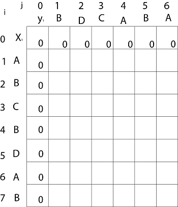
Example: Given two sequences X [1...m] and Y [1.....n]. Find the longest common subsequences to both.

here X = (A,B,C,B,D,A,B) and Y = (B,D,C,A,B,A)
     m = length [X] and n = length [Y]
     m = 7 and n = 6
Here x1= x [1] = A   y1= y [1] = B
     x2= B  y2= D 
     x3= C  y3= C
     x4= B  y4= A
     x5= D  y5= B
     x6= A  y6= A
     x7= B
Now fill the values of c [i, j] in m x n table
Initially, for i=1 to 7 c [i, 0] = 0
          For j = 0 to 6 c [0, j] = 0

That is:

Now for i=1 and j = 1
 x1 and y1 we get x1 ≠ y1 i.e. A ≠ B
And  c [i-1,j] = c [0, 1] = 0
 c [i, j-1] = c [1,0 ] = 0
That is, c [i-1,j]= c [i, j-1] so c [1, 1] = 0 and b [1, 1] = ' ↑  '

Now for i=1 and j = 2
x1 and y2 we get x1 ≠ y2 i.e. A ≠ D
 c [i-1,j] = c [0, 2] = 0
 c [i, j-1] = c [1,1 ] = 0
That is, c [i-1,j]= c [i, j-1] and c [1, 2] = 0 b [1, 2] = '  ↑  '

Now for i=1 and j = 3
 x1 and y3 we get x1 ≠ y3 i.e. A ≠ C
 c [i-1,j] = c [0, 3] = 0
 c [i, j-1] = c [1,2 ] = 0
so c [1,3] = 0     b [1,3] = ' ↑ '

Now for i=1 and j = 4
 x1 and y4 we get. x1=y4 i.e A = A 
  c [1,4] = c [1-1,4-1] + 1
     = c [0, 3] + 1
      = 0 + 1 = 1
 c [1,4] = 1
 b [1,4] = '  ↖  '

Now for i=1 and j = 5
           x1 and y5  we get x1 ≠ y5
           c [i-1,j] = c [0, 5] = 0
 c [i, j-1] = c [1,4 ] = 1
Thus c [i, j-1] >  c [i-1,j] i.e. c [1, 5] = c [i, j-1] = 1. So b [1, 5] = '←'

Now for i=1 and j = 6
           x1 and y6   we get x1=y6
                     c [1, 6] = c [1-1,6-1] + 1
                              = c [0, 5] + 1 = 0 + 1 = 1
     c [1,6] = 1
     b [1,6] = '  ↖  '

Now for i=2 and j = 1
 We get x2 and y1 B = B i.e.  x2= y1
             c [2,1] = c [2-1,1-1] + 1
                     = c [1, 0] + 1
                     = 0 + 1 = 1   
             c [2, 1] = 1 and b [2, 1] = ' ↖ '
Similarly, we fill the all values of c [i, j] and we get

Step 4: Constructing an LCS: The initial call is PRINT-LCS (b, X, X.length, Y.length)

PRINT-LCS (b, x, i, j)
 1. if i=0 or j=0
 2. then return
 3. if b [i,j] = ' ↖ '
 4. then PRINT-LCS (b,x,i-1,j-1)
 5. print x_i
 6. else if b [i,j] = '  ↑  '
 7. then PRINT-LCS (b,X,i-1,j)
 8. else PRINT-LCS (b,X,i,j-1)

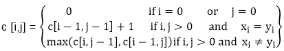
Example: Determine the LCS of (1,0,0,1,0,1,0,1) and (0,1,0,1,1,0,1,1,0).

Solution: let X = (1,0,0,1,0,1,0,1) and Y = (0,1,0,1,1,0,1,1,0).

We are looking for c [8, 9]. The following table is built.

From the table we can deduct that LCS = 6. There are several such sequences, for instance (1,0,0,1,1,0) (0,1,0,1,0,1) and (0,0,1,1,0,1)

Shortest path

1.  Floyd Warshall Algorithm 

The Floyd Warshall Algorithm is for solving the All Pairs Shortest Path problem. The problem is to find shortest distances between every pair of vertices in a given edge weighted directed Graph.

Example:

Input:
       graph[][] = { {0,   5,  INF, 10},
                    {INF,  0,  3,  INF},
                    {INF, INF, 0,   1},
                    {INF, INF, INF, 0} }
which represents the following graph
             10
       (0)------->(3)
        |         /|\
      5 |          |
        |          | 1
       \|/         |
       (1)------->(2)
            3       
Note that the value of graph[i][j] is 0 if i is equal to j 
And graph[i][j] is INF (infinite) if there is no edge from vertex i to j.

Output:
Shortest distance matrix
      0      5      8      9
    INF      0      3      4
    INF    INF      0      1
    INF    INF    INF      0 

1. Floyd Warshall Algorithm
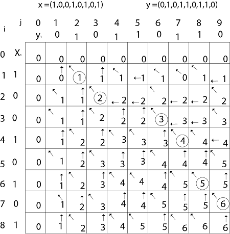
We initialize the solution matrix same as the input graph matrix as a first step. Then we update the solution matrix by considering all vertices as an intermediate vertex. The idea is to one by one pick all vertices and updates all shortest paths which include the picked vertex as an intermediate vertex in the shortest path. When we pick vertex number k as an intermediate vertex, we already have considered vertices {0, 1, 2, .. k-1} as intermediate vertices. For every pair (i, j) of the source and destination vertices respectively, there are two possible cases.
1) k is not an intermediate vertex in shortest path from i to j. We keep the value of dist[i][j] as it is.
2) k is an intermediate vertex in shortest path from i to j. We update the value of dist[i][j] as dist[i][k] + dist[k][j] if dist[i][j] > dist[i][k] + dist[k][j]

The following figure shows the above optimal substructure property in the all-pairs shortest path problem.

Following is implementations of the Floyd Warshall algorithm

// C Program for Floyd Warshall Algorithm #include<stdio.h>    // Number of vertices in the graph #define V 4    /* Define Infinite as a large enough value. This value will be used   for vertices not connected to each other */ #define INF 99999    // A function to print the solution matrix void printSolution(int dist[][V]);    // Solves the all-pairs shortest path problem using Floyd Warshall algorithm void floydWarshall (int graph[][V]) {     /* dist[][] will be the output matrix that will finally have the shortest        distances between every pair of vertices */     int dist[V][V], i, j, k;        /* Initialize the solution matrix same as input graph matrix. Or         we can say the initial values of shortest distances are based        on shortest paths considering no intermediate vertex. */     for (i = 0; i < V; i++)         for (j = 0; j < V; j++)             dist[i][j] = graph[i][j];        /* Add all vertices one by one to the set of intermediate vertices.       ---> Before start of an iteration, we have shortest distances between all       pairs of vertices such that the shortest distances consider only the       vertices in set {0, 1, 2, .. k-1} as intermediate vertices.       ----> After the end of an iteration, vertex no. k is added to the set of       intermediate vertices and the set becomes {0, 1, 2, .. k} */     for (k = 0; k < V; k++)     {         // Pick all vertices as source one by one         for (i = 0; i < V; i++)         {             // Pick all vertices as destination for the             // above picked source             for (j = 0; j < V; j++)             {                 // If vertex k is on the shortest path from                 // i to j, then update the value of dist[i][j]                 if (dist[i][k] + dist[k][j] < dist[i][j])                     dist[i][j] = dist[i][k] + dist[k][j];             }         }     }        // Print the shortest distance matrix     printSolution(dist); }    /* A utility function to print solution */ void printSolution(int dist[][V]) {     printf ("The following matrix shows the shortest distances"             " between every pair of vertices \n");     for (int i = 0; i < V; i++)     {         for (int j = 0; j < V; j++)         {             if (dist[i][j] == INF)                 printf("%7s", "INF");             else                 printf ("%7d", dist[i][j]);         }         printf("\n");     } }    // driver program to test above function int main() {     /* Let us create the following weighted graph             10        (0)------->(3)         |         /|\       5 |          |         |          | 1        \|/         |        (1)------->(2)             3           */     int graph[V][V] = { {0,   5,  INF, 10},                         {INF, 0,   3, INF},                         {INF, INF, 0,   1},                         {INF, INF, INF, 0}                       };        // Print the solution     floydWarshall(graph);     return 0; }

Output:

Following matrix shows the shortest distances between every pair of vertices
      0      5      8      9
    INF      0      3      4
    INF    INF      0      1
    INF    INF    INF      0

Time Complexity: O(V^3)

The above program only prints the shortest distances. We can modify the solution to print the shortest paths also by storing the predecessor information in a separate 2D matrix.
Also, the value of INF can be taken as INT_MAX from limits.h to make sure that we handle maximum possible value. When we take INF as INT_MAX, we need to change the if condition in the above program to avoid arithmetic overflow.

2. Bellman–Ford Algorithm 

Given a graph and a source vertex src in graph, find shortest paths from src to all vertices in the given graph. The graph may contain negative weight edges.

We have discussed Dijkstra’s algorithm for this problem. Dijkstra’s algorithm is a Greedy algorithm and time complexity is O(VLogV) (with the use of Fibonacci heap). Dijkstra doesn’t work for Graphs with negative weight edges, Bellman-Ford works for such graphs. Bellman-Ford is also simpler than Dijkstra and suites well for distributed systems. But time complexity of Bellman-Ford is O(VE), which is more than Dijkstra.

Recommended: Please solve it on “PRACTICE ” first, before moving on to the solution.

Algorithm
Following are the detailed steps.

Input: Graph and a source vertex src
Output: Shortest distance to all vertices from src. If there is a negative weight cycle, then shortest distances are not calculated, negative weight cycle is reported.

1) This step initializes distances from source to all vertices as infinite and distance to source itself as 0. Create an array dist[] of size |V| with all values as infinite except dist[src] where src is source vertex.

2) This step calculates shortest distances. Do following |V|-1 times where |V| is the number of vertices in given graph.
…..a) Do following for each edge u-v
………………If dist[v] > dist[u] + weight of edge uv, then update dist[v]
………………….dist[v] = dist[u] + weight of edge uv

3) This step reports if there is a negative weight cycle in graph. Do following for each edge u-v
……If dist[v] > dist[u] + weight of edge uv, then “Graph contains negative weight cycle”
The idea of step 3 is, step 2 guarantees shortest distances if graph doesn’t contain negative weight cycle. If we iterate through all edges one more time and get a shorter path for any vertex, then there is a negative weight cycle

How does this work? Like other Dynamic Programming Problems, the algorithm calculate shortest paths in bottom-up manner. It first calculates the shortest distances which have at-most one edge in the path. Then, it calculates shortest paths with at-most 2 edges, and so on. After the i-th iteration of outer loop, the shortest paths with at most i edges are calculated. There can be maximum |V| – 1 edges in any simple path, that is why the outer loop runs |v| – 1 times. The idea is, assuming that there is no negative weight cycle, if we have calculated shortest paths with at most i edges, then an iteration over all edges guarantees to give shortest path with at-most (i+1) edges (Proof is simple, you can refer this or MIT Video Lecture)

Example
Let us understand the algorithm with following example graph. The images are taken from this source.

Let the given source vertex be 0. Initialize all distances as infinite, except the distance to source itself. Total number of vertices in the graph is 5, so all edges must be processed 4 times.

Let all edges are processed in following order: (B, E), (D, B), (B, D), (A, B), (A, C), (D, C), (B, C), (E, D). We get following distances when all edges are processed first time. The first row in shows initial distances. The second row shows distances when edges (B, E), (D, B), (B, D) and (A, B) are processed. The third row shows distances when (A, C) is processed. The fourth row shows when (D, C), (B, C) and (E, D) are processed.

The first iteration guarantees to give all shortest paths which are at most 1 edge long. We get following distances when all edges are processed second time (The last row shows final values).

The second iteration guarantees to give all shortest paths which are at most 2 edges long. The algorithm processes all edges 2 more times. The distances are minimized after the second iteration, so third and fourth iterations don’t update the distances.

Thank you,
Er. Shejwal Shrikant.